Further examples of vector spaces

Polynomials

We introduce a number of further examples of vector spaces. Recall that a function \(f : {\bf R} \to {\bf R}\) (i.e., cf. §Chapter A, a function that takes as an input a real number \(x\) and whose output \(f(x)\) is another real number) is called a polynomial if it is of the form

\[ f(x) = a_n x^n + a_{n-1} x^{n-1} + \dots + a_1 x + a_0, \]

where \(a_n, a_{n-1}, \dots, a_0\) are real numbers. These numbers are called the coefficients of \(f\). The degree of \(f\) is the largest exponent \(n\) appearing in \(f\) (provided that the coefficient \(a_n \ne 0\)). Recall from §Chapter A that such an expression is abbreviated as

\[ f(x) = \sum_{i = 0}^n a_i x^i. \]

In increasing complexity, a constant function

\[ f(x) = a \]

is a polynomial of degree 0 (note \(a = a \cdot x^0\));

\[ f(x) = a_1 x + a_0 \]

is a linear polynomial (also known as linear function). Its degree is 1 (provided \(a_1 \ne 0\)). Next,

\[ f(x) = a_2 x^2 + a_1 x + a_0 \]

is called a quadratic polynomial (or quadratic function). Its degree is 2 (provided \(a_2 \ne 0\); if \(a_2 = 0\) then it is a linear polynomial). These types of functions are familiar from high-school.

Definition and Lemma 3.22 (Related exercises: Exercise 3.3, Exercise 3.9)

The set

\[ {\bf R}[x] := \{ f : {\bf R} \to {\bf R} \ | \ f \text{ is a polynomial} \} \]

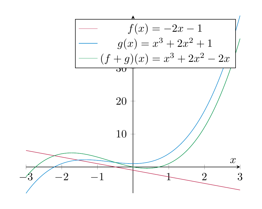
is a vector space, where we define the sum and scalar multiplication as follows: given two polynomials \(f, g \in P\), their sum is the function \(f + g : {\bf R} \to {\bf R}\)defined by

\[ (f + g)(x) := f(x) + g(x), \]

(3.23)

and given a real number \(r \in {\bf R}\), the scalar multiple is the function \(r f : {\bf R} \to {\bf R}\) defined by

\[ (r f)(x) := r \cdot f(x). \]

(3.24)

The set

\[ {\bf R}[x]^{\le d} := \{ \sum_{i = 0}^d a_i x^i \ | a_0, \dots, a_d \in {\bf R}\} (\subset {\bf R}[x]) \]

of polynomials of degree at most \(d\) is a subspace of \({\bf R}[x]\).

Proof. We have to check the conditions on a vector space (Definition 3.10). As it also happens often in other examples, the most notable condition to check is that the sum and scalar multiple is again an element of the vector space. Here, we need to check that for \(f, g \in P\) the function \(f + g\) defined above is again a polynomial. Fortunately, this is easy: if \(f(x) = a_n x^n + a_{n-1} x^{n-1} + \dots + a_1 x + a_0\) and \(g(x) = b_n x^n + b_{n-1} x^{n-1} + \dots + b_0\), then, by definition

\[ \begin{align*} (f+g)(x) & = a_n x^n + a_{n-1} x^{n-1} + \dots + a_0 + b_n x^n + b_{n-1} x^{n-1} + \dots + b_0 \\ & = a_n x^n + b_n x^n + a_{n-1} x^{n-1} + b_{n-1} x^{n-1} + \dots + a_0 + b_0 \\ & = \underbrace{(a_n + b_n)}_{=:c_n} x^n + \underbrace{(a_{n-1}+b_{n-1})}_{=:c_{n-1}} x^{n-1} + \dots + \underbrace{(a_0 + b_0)}_{=:c_0} \\ & = c_n x^n + c_{n-1} x^{n-1} + \dots + c_0. \end{align*} \]

Thus, the sum of \(f\) and \(g\) is another polynomial. Similarly, one verifies that the scalar multiple \(r \cdot f\) is a polynomial (check this! what are its coefficients?). With these checks done, one can proceed checking the remaining conditions in Definition 3.10. Checking this is comparatively uninsightful, and will be skipped.

Checking that \({\bf R}[x]^{\le d}\) is a subspace amounts to asserting that the 0 polynomial \(f(x) = 0\) has degree at most \(d\), and that sums and scalar (!) multiples of polynomials of degree \(\le d\) have again degree \(\le d\). This is clear. ◻

Remark 3.25

It is also true that the product of two polynomials is again a polynomial, but this is not part of what it takes to be a vector space, so we disregard that property at this point.

Remark 3.26

Instead of just polynomials, one can consider more general functions:

\[ \begin{align*} {\bf R}[x] & \subset \{ f : {\bf R} \to {\bf R} \ | \ f \text{ is differentiable } \} \\ & \subset \{ f : {\bf R} \to {\bf R} \ | \ \text{ is continuous } \} \\ & \subset\{ f : {\bf R} \to {\bf R} \text{ is any function} \} \end{align*} \]

are increasingly large vector spaces, cf. Exercise 3.3. The (huge!) space of all differentiable functions is a key player in analysis.

Direct sums

Definition and Lemma 3.27

Let \(V, W\) be two vector spaces. Their direct sum is the set

\[ V \oplus W := \{ (v, w) \ | \ v \in V, w \in W \}. \]

It is endowed with the addition given by

\[ (v, w) + (v', w') := (v+v', w+w') \]

and scalar multiplication given by

\[ r \cdot (v, w) := (rv, rw). \]

These operations turn \(V \oplus W\) into a vector space.

More generally, the same definition works for finitely many[^1] vector spaces \(V_1, \dots, V_n\), giving rise to the direct sum \(V_1 \oplus \dots \oplus V_n\).

This is easy to check: revisit the definition of a vector space and see how checking each of the 8 axioms for \(V \oplus W\) reduces to using the precise same axioms for \(V\) and \(W\). In particular, the zero vector in \(V \oplus W\) is the pair \((0_V, 0_W)\), where for clarity \(0_V\) denotes the zero vector in \(V\) and \(0_W\) the one in \(W\).

Example 3.28

We have \({\bf R}^2 = {\bf R} \oplus {\bf R}\) and in general

\[ {\bf R}^n = \underbrace{{\bf R} \oplus \dots \oplus {\bf R}}_{n \text{ summands}}. \]

This is clear from the definition of the sum of vectors in \({\bf R}^n\) (Definition 3.3) and the scalar multiplication (Definition 3.7).

Note that \(V \subset V \oplus W\), by regarding a vector \(v \in V\) as the vector \((v, 0_W)\). Likewise we can regard some \(w \in W\) as the vector \((0_V, w) \in V \oplus W\). This way, \(V \oplus W\) is a vector space that naturally contains both \(V\) and \(W\).

Example 3.29

The direct sum \({\bf R}^2 \oplus {\bf R}\) consists of pairs \((v, w)\) with \(v = (x, y) \in {\bf R}^2\) and \(w \in {\bf R}\). Thus, \({\bf R}^2 \oplus {\bf R} = \{((x,y), w) \ | \ x, y, w \in {\bf R}\}\). We can identify such a pair (consisting of a pair \((x,y)\) and a number \(w\)) with a triple \((x,y,w)\). Therefore, \({\bf R}^2 \oplus {\bf R}\) can be identified with \({\bf R}^3\). The sum and scalar multiple on \({\bf R}^2 \oplus {\bf R}\) as defined in Definition and Lemma 3.27 then reduce to the usual sum and scalar multiple in \({\bf R}^3\) as defined in Definition 3.3 and Definition 3.7.

Quotient spaces

All the examples of vector spaces that we have encountered so far were subspaces of an already given vector space, beginning with some ambient \({\bf R}^n\). However, not all vector spaces embed (naturally) in some \({\bf R}^n\). To illustrate this, we consider an example of a so-called quotient space. Since a full treatment of this would require a few more basic notions, we only discuss this in a special case:

Definition 3.30

Consider \(V = {\bf R}^2\), the plane, and a line \(L \subset W\) through the origin. We define a set

\[ V / L := \{ \text{ all lines that are parallel to } L \ \}. \]

(This is read “\(V\) modulo \(L\).”) For example, \(L_1\) and \(L_2\) are elements in that set \(V / L\) in the illustration below.

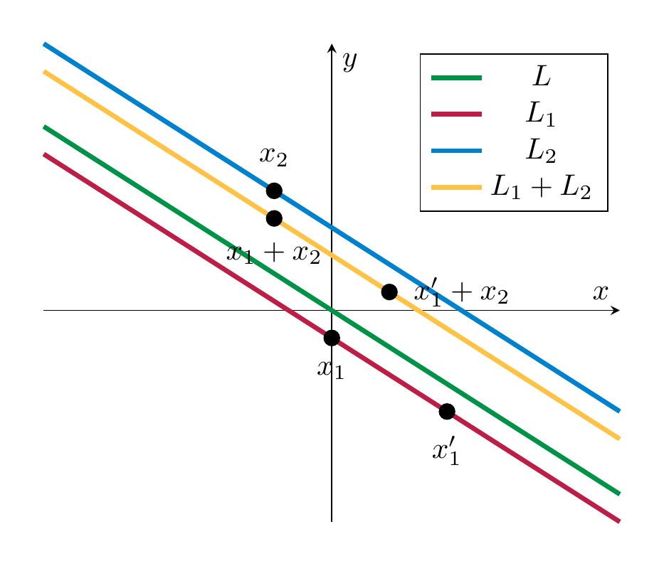
How to define the sum and scalar multiplication on that set \(V/L\)? Given \(L_1, L_2 \in V/L\), take any \(x_1 \in L_1\) and any \(x_2 \in L_2\). (These are both vectors in \(V = {\bf R}^2\).) Form the unique line that passes through \(x_1 + x_2\) and is parallel to \(L\). Call this line \(L_1 + L_2\). Similarly, the scalar multiple \(r \dot L_1\) is the line passing through \(r \cdot x_1\) and parallel to \(L\). What is remarkable is that makes sense, i.e., that the resulting lines do not depent on the choices of \(x_1, x_2\) above. In the illustration below, we indicate two choices for \(x_1\) (the second one being denoted \(x_1'\)). The sum \(x_1 + x_2\) is clearly different from \(x'_1 + x_2\), but they do lie on the same line (that is parallel to \(L\)). This holds since \(x'_1 - x_1\) lies in \(L\). Thus

\[ (x'_1 + x_2) - (x_1 + x_2) = x'_1 - x_1 \]

also lies in \(L\), and therefore \(x'_1 + x_2\) and \(x_1 + x_2\) lie on the same line that is parallel to \(L\).

With this settled, one can show (withouth much head-ache) that \(V/L\) is indeed a vector space. (What is the zero vector in \(V/L\)?)

A conceptually important insight is that there is no natural way in which this \(V/L\) is a subspace of \({\bf R}^2\). E.g., one may assign to an element \(L_1 \in V/L\), say, the \(y\)-coordinate of the intersection of \(L_1\) with the \(y\)-axis. But, this idea is ad-hoc and problem-laden (why not take the \(x\)-axis instead, and what is worse, what happens if \(L\) is in fact the \(y\)-axis...).

[^1]: or even infinitely many