Matrices associated to linear maps

In Proposition 4.19, we associated a linear map \({\bf R}^n \to {\bf R}^m\) to an \(m \times n\)-matrix. In this section, we will reverse this process: we will begin with a linear map and associate to it a matrix.

Proposition 4.44 (Related exercises: Exercise 4.15, Exercise 4.16, Exercise 4.3, Exercise 4.14, Exercise 4.21)

Let \(V, W\) be two vector spaces with bases \(v_1, \dots, v_n\) and \(w_1, \dots, w_m\), respectively. Let finally \(f: V \to W\) be a linear map. Then there is a unique \(m \times n\)-matrix \(A = (a_{ij})\), called the matrix associated to the linear map \(f\) with respect to the given bases, such that

\[ f(v_i) = \sum_{j=1}^m a_{ji} w_j. \]

We denote this matrix by

\[ {\mathrm M}_{f, \underline v, \underline w} := {\mathrm M}_{f, \{v_1, \dots, v_n\}, \{w_1, \dots, w_m\}} := (a_{ij}), \]

where for brevity \(\underline v := \{v_1, \dots, v_n\}\) and \(\underline w := \{w_1, \dots, w_m\}\).

For a general vector \(v = \sum_{i=1}^n b_i v_i\), we have

\[ f(v) = \sum_{i=1}^n \sum_{j=1}^m b_i a_{ji} w_j. \]

Proof. We apply the above fact (Proposition 3.64) to \(f(v_i) \in W\) (and the basis \(w_1, \dots, w_m\)), and see immediately that a unique expression of \(f(v_i)\) as claimed exists.

We now compute \(f(v)\):

\[ \begin{align*} f(v) & = f(\sum_{i=1}^n b_i v_i) \\ & = \sum_{i=1}^n b_i f(v_i) & \text{since }f \text{ is linear} \\ & = \sum_{i=1}^n b_i \sum_{j=1}^m a_{ji} w_j \\ & = \sum_{i=1}^n \sum_{j=1}^m b_i a_{ji} w_j. \end{align*} \]

◻

Example 4.45

We continue Example 4.43. The vectors \(w_1 = f(v_1) = (2,-1,0)\), \(w_2 = f(v_2) = (1,-1,1)\) and \(w_3 = f(v_3) = (0,2,2)\) form a basis of \({\bf R}^3\), as one sees by computing the rank of

\[ \left ( \begin{array}{ccc} 2 & -1 & 0 \\ 1 & -1 & 1 \\ 0 & 2 & 2 \end{array} \right ), \]

which is three. We can therefore apply Proposition 4.44 to the bases \(v_1, v_2, v_3\) and \(w_1, w_2, w_3\). The matrix is then

\[ \left ( \begin{array}{ccc} 1 & 0 & 0 \\ 0 & 1 & 0 \\ 0 & 0 & 1 \end{array} \right )! \]

To see this, note for example the second row says

\[ f(e_2) = 0 w_1 + 1 w_2 + 0 w_3, \]

which is true.

If, by contrast, we consider the standard basis \(e_1, e_2, e_3\) of \(V = {\bf R}^3\) (and still \(w_1, w_2, w_3\) in \(W = {\bf R}^3\)), then the matrix reads

\[ \left ( \begin{array}{ccc} 1 & 0 & 0 \\ 0 & 1 & 1 \\ 0 & 0 & -1 \end{array} \right ). \]

For example, the third column of this matrix expresses the identity

\[ f(e_3) = a_{13} w_1 + a_{23} w_2 + a_{33} w_3 = w_2 - w_3, \]

which we computed above.

This in particular shows that the matrix \(A\) depends (not only on \(f\) but also on) the choice of the bases of \(V\) and \(W\)!

Example 4.46

We consider the rotation matrix \(A = \left ( \begin{array}{cc} 0 & -1 \\ 1 & 0 \end{array} \right )\), cf. Example 4.17, and consider the associated linear map

\[ f : {\bf R}^2 \to {\bf R}^2, v = \left ( \begin{array}{c} x \\ y \end{array} \right ) \mapsto Av = \left ( \begin{array}{c} -y \\ x \end{array} \right ). \]

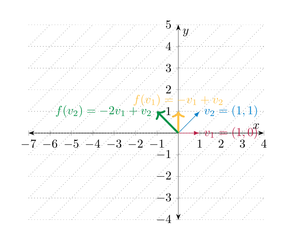
We consider the basis \(\underline v\) of \({\bf R}^2\) consisting of \(v_1 = (1, 0)\) and \(v_2 = (1, 1)\). We compute the basis of \(f\) with respect to \(\underline v\) on the domain \({\bf R}^2\), and the standard basis on the codomain \({\bf R}^2\). In order to compute it, we need to express \(v_1\) and \(v_2\) in terms of the standard basis, which is straightforward:

\[ \begin{align*} v_1 & = 1 \cdot e_1 + 0 \cdot e_2 \\ v_2 & = 1 \cdot e_1 + 1 \cdot e_2. \end{align*} \]

The linearity of \(f\) implies

\[ \begin{align*} f(v_1) & = 1 \cdot f(e_1) + 0 \cdot f(e_2) = \left ( \begin{array}{c} 0 \\ 1 \end{array} \right ) = \underbrace{0}_{a_{11}} \cdot e_1 + \underbrace{1}_{a_{21}} \cdot e_2. \\ f(v_2) & = 1 \cdot f(e_1) + 1 \cdot f(e_2) = \left ( \begin{array}{c} 0 \\ 1 \end{array} \right ) + \left ( \begin{array}{c} -1 \\ 0 \end{array} \right ) = \left ( \begin{array}{c} -1 \\ 1 \end{array} \right ) = \underbrace{-1}_{a_{12}} \cdot e_1 + \underbrace{1}_{a_{22}} \cdot e_2. \\. \end{align*} \]

Thus, the matrix of \(f\) with respect to afore-mentioned bases is

\[ A = \left ( \begin{array}{cc} a_{11} & a_{12} \\ a_{21} & a_{22} \end{array} \right ) = \left ( \begin{array}{cc} 0 & -1 \\ 1 & 1 \end{array} \right ). \]

We additionally compute the matrix of \(f\) with respect to the basis \(\underline v\) both on the domain and on the codomain. To this end, we need to express the vectors \(\left ( \begin{array}{c} 0 \\ 1 \end{array} \right )\) and \(\left ( \begin{array}{c} -1 \\ 1 \end{array} \right )\) as linear combinations of \(v_1\) and \(v_2\). We have

\[ \begin{align*} \left ( \begin{array}{c} 0 \\ 1 \end{array} \right ) & = -v_1 + v_2 \\ \left ( \begin{array}{c} -1 \\ 1 \end{array} \right ) & = -2v_1 + v_2. \end{align*} \]

Thus, the matrix of \(f\) with respect to the basis \(\underline v\) on both the domain and the codomain is

\[ \left ( \begin{array}{cc} -1 & -2 \\ 1 & 1 \end{array} \right ). \]