Definition of vector spaces¶

Definition 3.10 (Related exercises: Exercise 3.1)

A vector space is a set \(V\) that is equipped with two functions called the sum and the scalar multiplication:

\[ \begin{align*} + : & \ V \times V \to V, (v, w) \mapsto v + w,\\ \cdot : & \ {\bf R} \times V \to V, (r, v) \mapsto rv \text{ (or }r\cdot v \text{)} \end{align*} \]

satisfying the following conditions. Below \(r, s \in {\bf R}\) are arbitrary real numbers and \(u, v, w \in V\) arbitrary elements of \(V\) (also referred to as vectors):

\(v+ w= w+v\) (commutativity of addition),
\(u+(v+w) = (u+v)+w\),
there is a vector \(0 \in V\), called the zero vector, such that \(0 + v = v\) for all \(v \in V\),
\(r(v+w) = rv+rw\) (distributive law),
\((r+s)v = rv+sv\),
\((rs)v = r(sv)\),
\(1 v = v\),
\(0 v = 0\) (at the left 0 denotes the real number zero, at the right it denotes the zero vector)

Example 3.11

The sets \({\bf R} = {\bf R}^1\), \({\bf R}^2\), and in general \({\bf R}^n\) are vector spaces (where the function \(+\) is given by vector addition and \(\cdot\) is scalar multiplication). Indeed, the conditions in Definition 3.10 are precisely the properties of vector addition and scalar multiplication noted before in Lemma 3.6 and Lemma 3.9.

Remark 3.12

Recall from §Chapter A that the notation appearing in

\[ + : V \times V \to V, (v, w) \mapsto v + w \]

means that \(+\) is a function that takes as an input two elements in \(V\), which here are denoted \(v\) and \(w\), and produces as an output another element in \(V\). That element is denoted \(v + w\). Likewise

\[ \cdot : {\bf R} \times V, (r, v) \mapsto rv \text{ (or }r\cdot v \text{)} \]

means that \(\cdot\) is a function whose input is a pair consisting of a real number, here denoted \(r\), and an element in \(V\), and produces as an output an element in \(V\) that is denoted \(rv\) or \(r \cdot v\).

Some authors distinguish notationally between vectors and numbers by writing \(\vec v\) for vectors and \(r\) for numbers. In these notes, we usually do not use that convention.

Example 3.13

The following subsets of \({\bf R}^n\) are not vector spaces. In each case, draw the set and point out precisely which of the above condition(s) fails.

\(\{(x_1, x_2) \in {\bf R}^2 \text{ with }x_1 \ge 0\}\),
\(\{(x_1, x_2) \in {\bf R}^2 \text{ with }x_1 \ne 0\}\),
The solution set of the equation

\[ 3x_1 + 2x_2 = 3. \]

\(\{(x_1, x_2) \in {\bf R}^2 \text { with }x_1 = 0 \text{ or } x_2 = 0 \}\).

Solution sets of homogeneous linear systems¶

Recall from Definition 2.13 that a homogeneous linear system is one on which the constant terms are all zero, i.e., one of the form

\[ \begin{align} a_{11} x_1 + a_{12} x_2 + \dots + a_{1n} x_n & = 0 \\ a_{21} x_1 + a_{22} x_2 + \dots + a_{2n} x_n & = 0 \nonumber \\ \vdots \nonumber\\ a_{m1} x_1 + a_{m2} x_2 + \dots + a_{mn} x_n & = 0 \nonumber \end{align} \]

(3.14)

In this section, we will see that the solution sets to homogeneous linear systems are vector spaces, which is an extremely important class of examples. We begin by looking at homogeneous linear equations, i.e., a linear system consisting of a single (homogeneous) equation.

Example 3.15

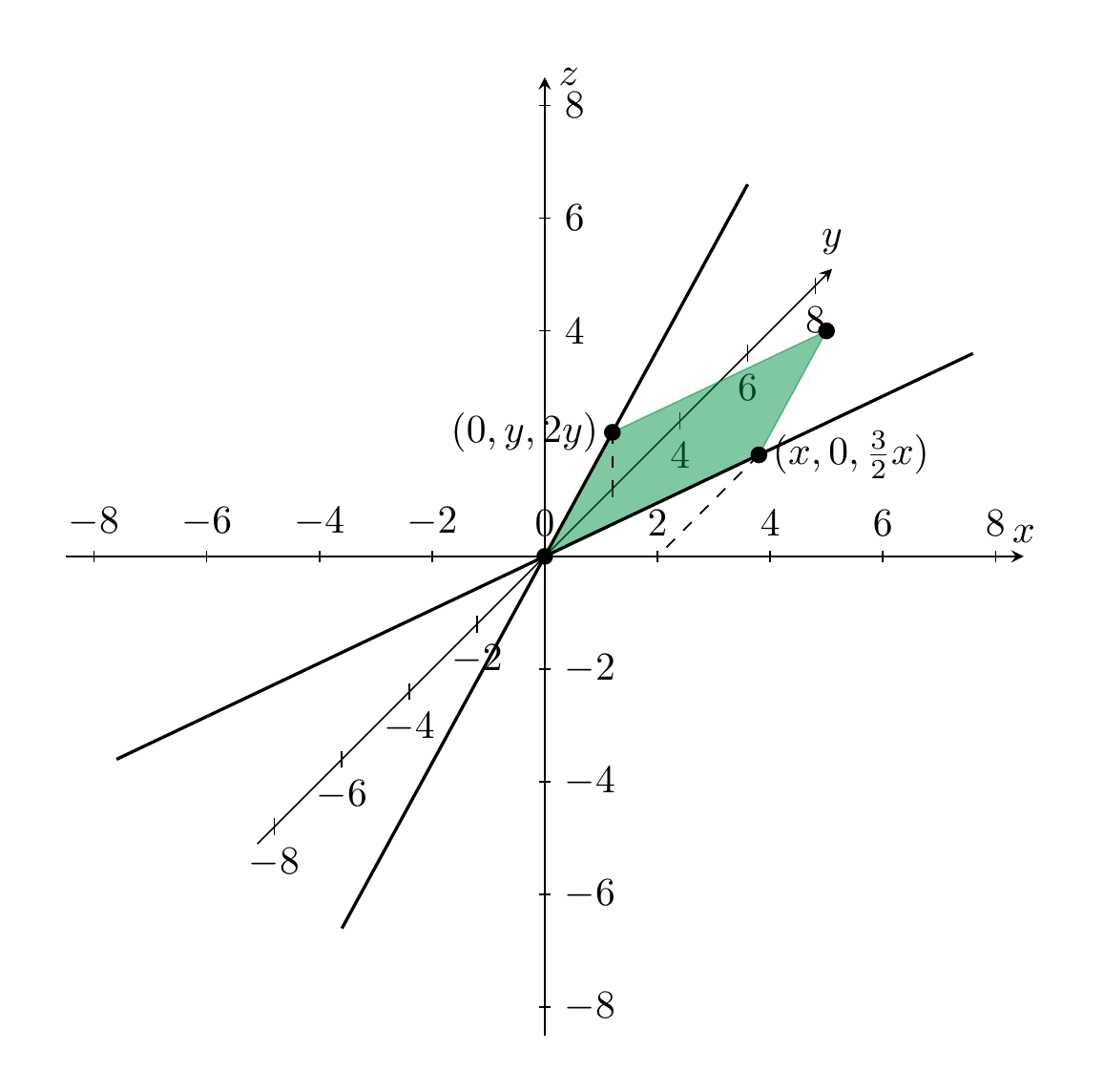
The homogeneous linear equation

\[ 3x + 4y - 2z = 0 \]

has the solution set

\[ \{(x, y, \frac{3x+4y}2) \ | \ x, y \in {\bf R} \}. \]

Indeed, a triple \((x,y,z)\) is a solution to the equation above precisely if \(z = \frac{3x+4y}2\), and \(x\) and \(y\) can be arbitrary real numbers. A few concrete elements in this solution set, drawn below, are the points \((0,0,0)\), \((2,0,3)\), \((0,1,2)\). Slightly more generally, triples of the form \((0, y, 2y)\) and \((x, 0, \frac 32 x)\), for arbitrary \(y\), resp. \(x\), are elements in the solution set. These lines (which lie in the \(y-z\)-plane, resp. in the \(x-y\)-plane) are also drawn below. Of course, the solution set contains further elements such as the point \((2,1,5)\). The green shape is meant to illustrate further elements of the solution set, but of course this is not bounded by the lines in the illustration, instead it stretches out in all directions.

Example 3.16

What equation (in the three variables \(x\), \(y\) and \(z\)) has the following solution set? Again the picture only shows the solution set partly, it is meant to be extended to the left and below.

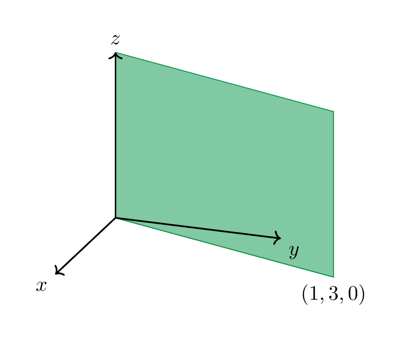
We note that both equations have a solution set which is a plane passing through the origin, i.e., the point \((0,0,0)\). We will want to articulate that this plane is a vector space that lies inside the larger ambient vector space \({\bf R}^3\).

Definition 3.17 (Related exercises: Exercise 3.3, Exercise 4.11, Exercise 4.12, Exercise 3.24, Exercise 3.9, Exercise 3.2)

A subspace (or sub-vector space, or vector subspace) \(V\) of \({\bf R}^n\) is a subset that is – in its own right – a vector space. I.e.,

it contains the zero vector,
for all vectors \(v, w \in V\), the sum \(v+w\) is an element of \(V\), and
for all \(v \in V\) and all real numbers \(r \in {\bf R}\), the scalar multiple \(r \cdot v\) is required to be an element of \(V\).

More generally, a subset \(V\) of another vector space \(W\) is a subspace if \(V\) satisfies the three preceeding conditions.

We have seen in Example 3.13 a number of subsets of \({\bf R}^2\) that fail to be subspaces. In particular, the solution set of the equation \(3x_1 + 2x_2 = 3\) is not a vector space since the zero vector \((0,0)\) is not a solution of this equation. This is not a homogeneous equation (the constant term is 3, but not 0). The next proposition tells us that this is the cause of the failure:

Proposition 3.18 (Related exercises: Exercise 3.22, Exercise 3.17, Exercise 3.14, Exercise 2.15, Exercise 2.14, Exercise 3.29)

Consider a homogeneous linear system in \(n\) variables \(x_1, \dots, x_n\), and \(m\) equations, as in Equation (3.14). Its solution set is a subspace of \({\bf R}^n\).

Proof. Let us call \(S\) the solution set of the system. I.e., an element \(x = (x_1, \dots, x_n)\) belongs to \(S\) precisely if it is a solution of the linear system Equation (3.14).

We check the three conditions in Definition 3.17:

\((0, \dots, 0) \in S\), i.e. the zero vector in \({\bf R}^n\) is a solution. Indeed, plugging in zero in all the \(x_i\) gives \(0 = 0\) for all the \(m\) equations, which holds.
Let \(v = (v_1, \dots, v_n)\) and \(w = (w_1, \dots, w_n)\) be elements of \(S\). We need to check that \(v + w\) is also in \(S\). Recall from Definition 3.3 that \(v + w = (v_1 + w_1, \dots, v_n + w_n)\). The \(m\) equations of the linear system read

\[ a_{i1} x_1 + a_{i2} x_2 + \dots + a_{in} x_n = 0, \]

where \(i = 1, \dots, m\). Inserting \(v_1 + w_1\) for \(x_1\) etc., we get

\[ \begin{align*} & a_{i1} (v_1 + w_1) + a_{i2} (v_2 + w_2) + \dots + a_{in} (v_n + w_n) \\ = & a_{i1} v_1 + a_{i1} w_1 + a_{i2} v_2 + a_{i2} w_2 + \dots + a_{in} v_n + a_{in} w_n \\ = & \underbrace{a_{i1} v_1 + a_{i2} v_2 + \dots + a_{in} v_n}_{=0} + \underbrace{a_{i1} w_1 + a_{i2} w_2 + \dots + a_{in} w_n}_{=0} \\ = & 0 + 0 \\ = & 0. \end{align*} \]

This shows that \(v + w \in S\).

In a similar manner, one shows (do it!) that for any \(r \in {\bf R}\) and \(v = (v_1, \dots, v_n) \in S\) the scalar multiple \(rv = (r v_1, \dots, rv_n)\) is again in \(S\).

◻