Vector spaces

\({\bf R}^2\), \({\bf R}^3\) and \({\bf R}^n\)

Definition 3.1

For \(n \ge 1\), an ordered \(n\)-tuple of real numbers is a collection of \(n\) real numbers in a fixed order. For \(n = 2\), an ordered 2-tuple is usually called an ordered pair, and an ordered 3-tuple is called an ordered triple. If these numbers are \(r_1, r_2, \dots, r_n\), then the ordered \(n\)-tuple consisting of these numbers is denoted

\[ (r_1, r_2, \dots, r_n). \]

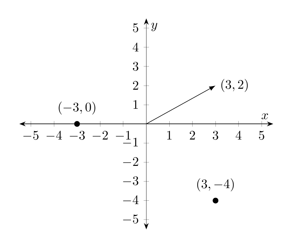
For example, \((2, 3)\) is an (ordered) pair. This pair is different from the (ordered) pair \((3, 2)\). It makes good sense to insist on the ordering, e.g., if a pair consists of the information

\[ (\text{``weight of a parcel (in kg)'', ``prize (in €)''}), \]

then \((3, 10)\) is of course different from \((10, 3)\). \((\frac 3 4, \sqrt 2, -7)\), \((0,0, 0)\) are examples of (ordered) 3-tuples. An ordered 1-tuple is simply a single real number.

Definition 3.2

For \(n \ge 1\), the set \({\bf R}^n\) is the set of all ordered \(n\)-tuples of real numbers. Thus (see §Chapter A for general mathematical notation)

\[ {\bf R}^n = \{ (r_1, r_2, \dots, r_n) \ | \ r_1, r_2, \dots, r_n \in {\bf R} \}. \]

Thus, \({\bf R}^1 = {\bf R}\) is just the set of real numbers. Next, \({\bf R}^2\) is the set of ordered pairs of real numbers:

\[ {\bf R}^2 = \{(r_1, r_2) \ | \ r_1, r_2 \in {\bf R} \}. \]

Of course, here \(r_1, r_2\) are just symbols which have no meaning in themselves, so we can also write

\[ \begin{align*} {\bf R}^2 & = \{(x_1, x_2) \ | \ x_1, x_2 \in {\bf R} \} \\ & = \{(x,y) \ | \ x, y \in {\bf R} \}. \end{align*} \]

The elements in \({\bf R}^n\) are also referred to as vectors. Thus, a vector is nothing but an ordered \(n\)-tuple. The element \((0, 0, \dots, 0) \in {\bf R}^n\) is called the zero vector. Instead of writing \((x_1, \dots, x_n)\) we also abbreviate this as \(x\), so that the expression

\[ x \in {\bf R}^n \]

means that \(x\) is an (ordered) \(n\)-tuple consisting of \(n\) real numbers \(x_1, \dots, x_n\). The numbers \(x_1\) etc. are called the components of the vector \(x\).

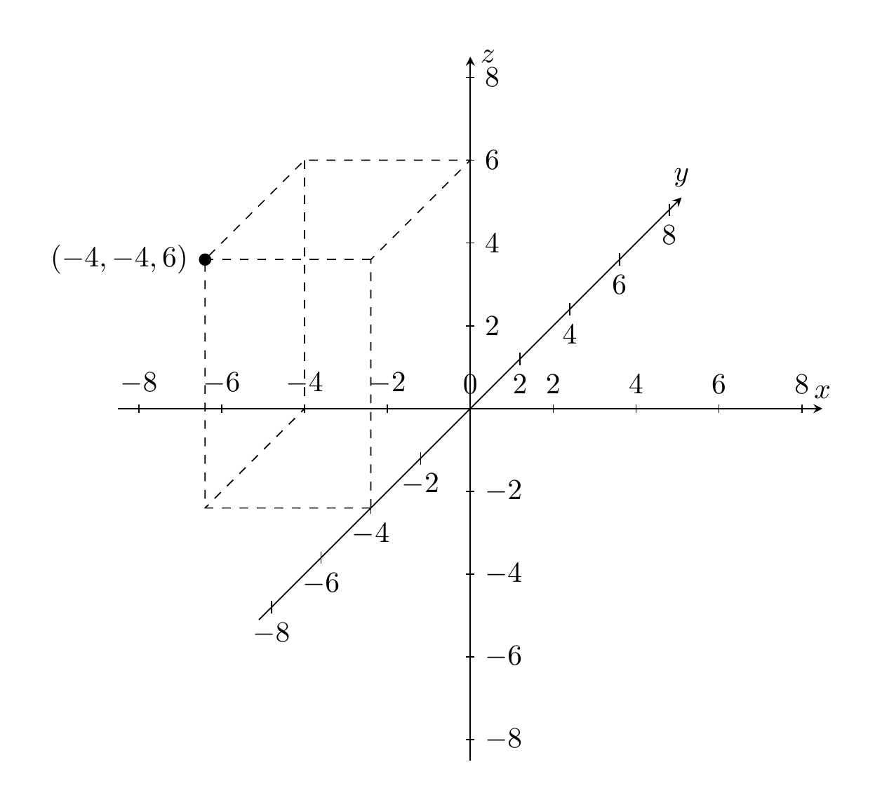
Vectors in \({\bf R}\), \({\bf R}^2\) and \({\bf R}^3\) can be visualized nicely as points on the real line, as points in the plane or as points in 3-dimensional space. It is also common to decorate vectors with an arrow, with the idea of representing a movement or relocation to that point, or in physics a force with a certain strength in a certain direction.

This visualization also helps explain some of the fundamental features of \({\bf R}^n\).

Addition of vectors

Definition 3.3

Given two vectors (in the same \({\bf R}^n\), i.e., having the same number of components)

\[ x = (x_1, \dots, x_n) \text{ and } y = (y_1, \dots, y_n) \in {\bf R}^n, \]

their sum is the vector

\[ (x_1 + y_1, x_2 + y_2, \dots, x_n + y_n). \]

Example 3.4

What is the sum of \((1,1)\) and \((-2, 1)\)? Visualize that sum graphically!

Remark 3.5

The sum of two vectors is only defined if they belong to the same \({\bf R}^n\): a sum such as \((1,2) + (3, 4, 5)\) is undefined, i.e. is a meaningless expression.

The sum of vectors has the following crucial properties:

Lemma 3.6

For \(x = (x_1, \dots, x_n), y = (y_1, \dots, y_n)\) and \(z = (z_1, \dots, z_n) \in {\bf R}^n\) the following rules hold:

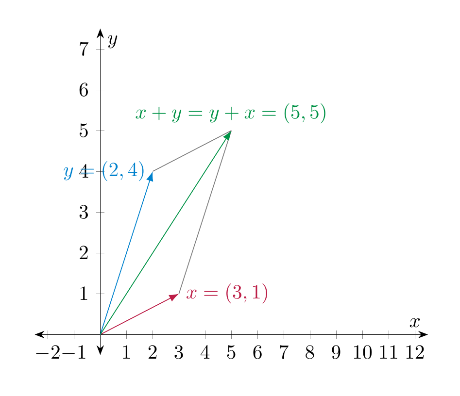
• \(x + y = y + x\) (commutativity of addition)

• \(x + 0 = x\) (adding the zero vector does not change the vector in question)

• \(x + (y+z) = (x+y) + z\) (associativity of addition)

These identities are easy to prove since they quickly boil down to similar identities for the sum of real numbers. Here is a visual intuition for the commutativity of addition, which is also called the parallelogram law.

Scalar multiplication of vectors

Definition 3.7

Given a vector \(x = (x_1, \dots, x_n) \in {\bf R}^n\) and a real number \(r \in {\bf R}\), the scalar multiplication of \(x\) by \(r\) is the vector

\[ r \cdot x := (r \cdot x_1, \dots, r \cdot x_n). \]

I.e., every component of \(x\) gets multiplied by the number \(r\). Often one just writes \(rx\) instead of \(r \cdot x\).

Geometrically, the scalar multiplication corresponds to stretching the vector \(x\) by the factor \(r\) (i.e., if \(r > 1\) it is stretching, for \(0 < r < 1\) it compresses the vector, for \(r < 0\) it additionally flips the direction of the vector).

Example 3.8

What is \(4 \cdot (-1, 3)\)? What is \((- \frac 14) \cdot (-1,3)\)? Visualize the vector \((-1,3)\) and these results graphically!

Note that in contrast to the sum of vectors the scalar multiplication combines two different entities: a real number and a vector. The scalar multiplication has the following key properties:

Lemma 3.9

For two real numbers \(r, s \in {\bf R}\) and two vectors \(x, y \in {\bf R}^n\), the following identities hold:

1. \(r(x+y) = rx+ry\) (distributivity law)

2. \((r+s)x = rx + sy\) (distributivity law)

3. \((rs)x = r(sx)\) (scalar multiplication with a product \(rs\) of two real numbers can be computed by first multiplying with \(s\) and then with \(r\))

4. \(1 x = x\) (scalar multiplication by 1 does not change the vector)

5. \(0 x = 0\) (scalar multiplication by 0 gives the zero vector)

Again, these identities are easy to check using that the same rules hold if \(x, y\) were just real numbers.