Multiplication of a matrix with a vector

In this section, we define the multiplication of a matrix with a vector and show how this gives rise to a linear map. This is an extremely important way to construct linear maps.

Definition 4.9 (Related exercises: Exercise 4.1, Exercise 4.2)

Let \(A = (a_{ij})_{1 \le i \le m, 1 \le j \le n}\) (cf. Notation 2.22) be an \(m \times n\)-matrix and \(v = \left ( \begin{array}{c} v_1 \\ \vdots \\ v_n \end{array} \right )\) be a \(n \times 1\)-matrix, i.e., a row vector with \(n\) columns. The product of \(A\) with \(v\) is the \(m \times 1\)-vector

\[ A v := \left ( \begin{array}{c} a_{11} v_1 + a_{12} v_2 + \dots + a_{1n} v_n \\ \vdots \\ a_{m1} v_1 + a_{m2} v_2 + \dots + a_{mn} v_n \end{array} \right ). \]

Thus, the \(i\)-th entry of the (column) vector \(Av\) is computed by traversing the \(i\)-th row of \(A\) and multiplying each entry of that row with the corresponding entry of \(v\).

Example 4.10

Here are two concrete examples:

\[ \begin{align*} \left ( \begin{array}{cc} 4 & -1 \\ 2 & 1 \\ 0 & -2 \end{array} \right ) \left ( \begin{array}{c} 3 \\ 4 \end{array} \right ) & = \left ( \begin{array}{c} 4 \cdot 3 - 1 \cdot 4 \\ 2 \cdot 3 +1 \cdot 4 \\ 0 \cdot 3 - 2 \cdot 4 \end{array} \right ) = \left ( \begin{array}{c} 8 \\ 10 \\ -8 \end{array} \right ).\\ \left ( \begin{array}{ccc} 1 & 3 & -2 \\ 0 & 1 & 0 \\ 1 & 0 & -1 \end{array} \right ) \left ( \begin{array}{c} 1 \\ 2 \\ -1 \end{array} \right ) & = \left ( \begin{array}{c} 1 \cdot 1 + 3 \cdot 2 + (-2) \cdot (-1) \\ {} \\ \end{array} \right ) = \left ( \begin{array}{c} 9 \\ {} \\ \end{array} \right ). \end{align*} \]

It makes perfectly good sense to consider matrices whose entries are variables. Compute:

\[ \left ( \begin{array}{ccc} 1 & 3 & -2 \\ 0 & 1 & 0 \\ 1 & 0 & -1 \end{array} \right ) \left ( \begin{array}{c} x \\ y \\ z \end{array} \right ) = \left ( \begin{array}{c} 1 \cdot x + 3 \cdot y + (-2) \cdot z \\ {} \\ \end{array} \right ) = \left ( \begin{array}{c} x+3y-2z \\ {} \\ \end{array} \right ). \]

Thus, the equation (of column vectors consisting of 3 rows)

\[ \left ( \begin{array}{ccc} 1 & 3 & -2 \\ 0 & 1 & 0 \\ 1 & 0 & -1 \end{array} \right ) \left ( \begin{array}{c} x \\ y \\ z \end{array} \right ) = \left ( \begin{array}{c} 3 \\ 4 \\ -2 \end{array} \right ) \]

is a very convenient way to write down the linear system

\[ \begin{align*} x + 3y-2z & = 1 \\ y & = 4 \\ x - z & = -2. \end{align*} \]

This shows that the product of matrices with column vectors is very useful in enconding linear systems. We record this observation in the due generality:

Observation 4.11

Let

\[ A = \left ( \begin{array}{ccc} a_{11} & \dots & a_{1n} \\ \vdots & \ddots & \vdots \\ a_{m1} & \dots & a_{mn} \end{array} \right ) \]

be an \(m \times n\)-matrix and

\[ x = \left ( \begin{array}{c} x_1 \\ \vdots \\ x_n \end{array} \right ) \]

be a column vector with \(n\) rows and

\[ b = \left ( \begin{array}{c} b_1 \\ \vdots \\ b_m \end{array} \right ) \]

be a column vector with \(m\) rows. Then the equation

\[ A x = b \]

is equivalent to the linear system (in the unknowns \(x_1, \dots, x_n\), consisting of \(m\) equations)

\[ \begin{align*} a_{11} x_1 + \dots + a_{1n} x_n & = b_1 \\ \vdots \\ a_{m1} x_1 + \dots + a_{mn} x_n & = b_m. \\ \end{align*} \]

The case of \(2 \times 2\)-matrices

The process of multiplying a matrix with a column vector is also geometrically very important. We now investigate this in more detail in the case where

\[ A = \left ( \begin{array}{cc} a_{11} & a_{12} \\ a_{21} & a_{22} \end{array} \right ) \in {\mathrm {Mat}}_{2 \times 2}. \]

For a column vector \(v = \left ( \begin{array}{c} v_1 \\ v_2 \end{array} \right )\) the product is, according to Definition 4.9,

\[ Av = \left ( \begin{array}{c} a_{11} v_1 + a_{12} x_2 \\ a_{21} v_1 + a_{22} v_2 \end{array} \right ). \]

\[ Av = \left ( \begin{array}{c} a_{11} v_1 + a_{12} x_2 \\ a_{21} v_1 + a_{22} v_2 \end{array} \right ). \]

(4.12)

In keeping with traditional notation from geometry, we will instead write the vector \(v\) as \(\left ( \begin{array}{c} x \\ y \end{array} \right )\), in which case

\[ Av = \left ( \begin{array}{c} a_{11} x + a_{12} y \\ a_{21} x + a_{22} y \end{array} \right ). \]

It is useful to organize this situation into a function, namely the function that sends the vector \(v\) to the vector \(Av\). We obtain a function

\[ f : {\bf R}^2 \to {\bf R}^2, v \mapsto Av \ \text{(read ``$v$ maps to $Av$''.)} \]

Of course, since \(Av\) depends on the entries of \(A\), so does this function \(f\).

Reflections

Example 4.13

We consider \(A = \left ( \begin{array}{cc} 1 & 0 \\ 0 & -1 \end{array} \right )\). According to the above we have

\[ Av = \left ( \begin{array}{c} x \\ -y \end{array} \right ). \]

We plot a few points \(v\) and the corresponding \(Av\):

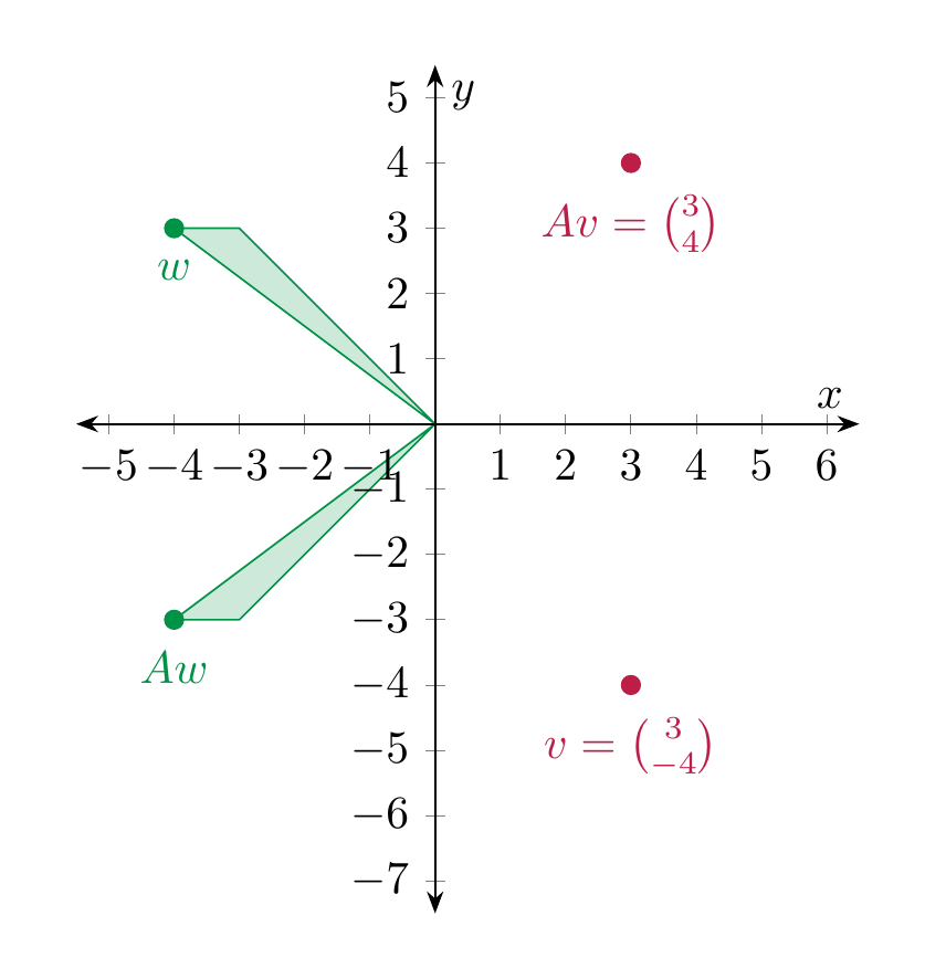
Thus, geometrically, \(Av\) is the point \(v\) reflected along the \(x\)-axis.

Rescalings

Example 4.14

The matrix \(A = \left ( \begin{array}{cc} \frac 12 & 0 \\ 0 & 1 \end{array} \right )\) describes the map that compresses everything in the \(x\)-direction by the factor \(\frac 12\), and leaves the \(y\)-direction untouched.

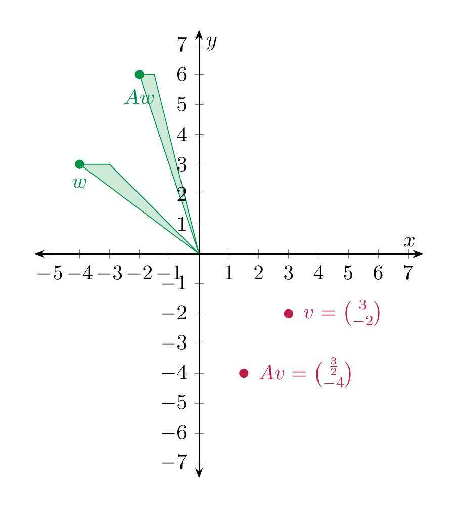
Example 4.15

If \(r\), \(s\) are two real numbers,

\[ A = \left ( \begin{array}{cc} r & 0 \\ 0 & s \end{array} \right ) \]

rescales the \(x\)-direction by a factor \(r\) (so it shrinks for \(r < 1\) and enlarges for \(r > 1\)) and rescales the \(y\)-direction by a factor \(s\).

For \(A = \left ( \begin{array}{cc} \frac 12 & 0 \\ 0 & 2 \end{array} \right )\), this looks as follows:

Shearing

Example 4.16

For a fixed real number \(r\), the matrix

\[ A = \left ( \begin{array}{cc} 1 & r \\ 0 & 1 \end{array} \right ) \]

sends \(v\) to \(Av = \left ( \begin{array}{c} x+ry \\ y \end{array} \right )\). Thus it is a shearing operation. In the following picture \(A = \left ( \begin{array}{cc} 1 & 2 \\ 0 & 1 \end{array} \right )\).

Rotations

We now consider rotations.

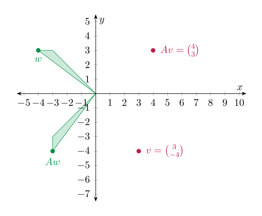
Example 4.17 (Related exercises: Exercise 4.1, Exercise 4.2)

For \(A = \left ( \begin{array}{cc} 0 & -1 \\ 1 & 0 \end{array} \right )\), the vector \(Av = \left ( \begin{array}{c} -y \\ x \end{array} \right )\). Geometrically, the function \(v \mapsto Av\) is a counterclockwise rotation by \(90^\circ\).

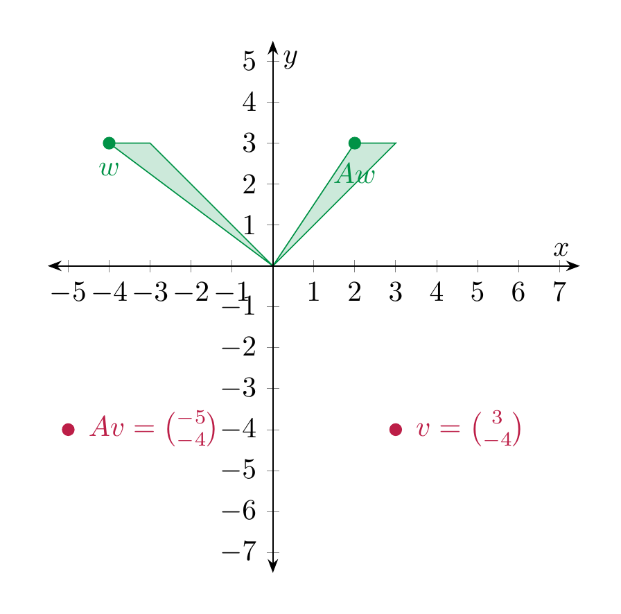
For \(A = \left ( \begin{array}{cc} -1 & 0 \\ 0 & 1 \end{array} \right )\), the vector \(Av = \left ( \begin{array}{c} -x \\ y \end{array} \right )\) so the function \(v \mapsto Av\) describes a counterclockwise rotation by \(180^\circ\) (or, what is the same, a clockwise rotation by \(180^\circ\)).

For more general rotations, we use basic properties of the trignometric functions, e.g., as recalled in §Chapter B.

Example 4.18 (Related exercises: Exercise 4.1)

In general, for any \(r \in {\bf R}\) the matrix

\[ A = \left ( \begin{array}{cc} \cos r & -\sin r \\ \sin r & \cos r \end{array} \right ) \]

is such that the function

\[ v \mapsto Av = \left ( \begin{array}{c} \cos r x - \sin r y \\ \sin r x + \cos r y \end{array} \right ) \]

is a (counter-clockwise) rotation by \(r\). For this reason, \(A\) is called a rotation matrix.

In the following illustration, \(A = \left ( \begin{array}{cc} 0 & -1 \\ 1 & 0 \end{array} \right )\).

We regard a vector \(v = \left ( \begin{array}{c} v_1 \\ \vdots \\ v_n \end{array} \right )\) as an element of \({\bf R}^n\). (Thus, instead of using the notation \((v_1, \dots, v_n)\) for an ordered tuple, as in Definition 3.1, we write the \(n\) numbers underneath in a row.) Fix an \(m \times n\)-matrix \(A\). Then the product \(Av\), which is an column vector with \(m\) entries, is an element in \({\bf R}^m\). We now regard this matrix \(A\) as fixed, and consider the vector \(v\) as a variable. In other words, we consider the function (or map)

\[ {\bf R}^n \to {\bf R}^m, v \mapsto A v. \]

Matrix multiplication has the following basic, but crucial property.

Proposition 4.19 (Related exercises: Exercise 4.17, Exercise 4.5, Exercise 4.21, Exercise 4.22)

For any \(m \times n\)-matrix \(A\), the above map is linear.

Proof. We prove this in the case \(m = n = 2\) using . (The case of general \(m\) and \(n\) is just notationally more involved, but otherwise the same.) Let \(v = \left ( \begin{array}{c} v_1 \\ v_2 \end{array} \right )\), \(v' = \left ( \begin{array}{c} v'_1 \\ v'_2 \end{array} \right )\). Then

\[ \begin{align*} A v + A v' & = \left ( \begin{array}{c} a_{11} v_1 + a_{12} v_2 \\ a_{21} v_1 + a_{22} v_2 \end{array} \right ) + \left ( \begin{array}{c} a_{11} v'_1 + a_{12} v'_2 \\ a_{21} v'_1 + a_{22} v'_2 \end{array} \right ) \\ & = \left ( \begin{array}{c} a_{11} (v_1+v'_1) + a_{12} (v_2+v'_2) \\ a_{21} (v_1+v'_1) + a_{22} (v_2+v'_2) \end{array} \right ) \\ & = A \left ( \begin{array}{c} v_1+v_2 \\ v'_1 + v'_2 \end{array} \right ) \\ & = A (v+v'). \end{align*} \]

Likewise, one checks Equation (4.3), i.e., that for \(a \in R\),

\[ \begin{align*} A (av) &= A \left ( \begin{array}{c} av_1 \\ a v_2 \end{array} \right ) \\ & = \left ( \begin{array}{c} a_{11} a v_1 + a_{12} a v_2 \\ a_{21} a v_1 + a_{22} a v_2 \end{array} \right ) \\ & =a \left ( \begin{array}{c} a_{11} v_1 + a_{12} v_2 \\ a_{21} v_1 + a_{22} v_2 \end{array} \right ) \\ & = a A v \\ & = a (A v). \end{align*} \]

◻