Composing linear maps and multiplying matrices

The following lemma, while simple to prove, is of fundamental importance:

Definition and Lemma 4.47

Let \(f : U \to V\) and \(g: V \to W\) be two linear maps between three vector spaces \(U\), \(V\) and \(W\). Then the composition of \(g\) and \(f\) is the map defined as

\[ g \circ f : U \to W, u \mapsto g(f(u)). \]

This map is again linear.

Proof. We check the two conditions in Definition 4.1: for \(u, u' \in U\) and \(a \in {\bf R}\), we have, using the linearity of \(f\) and \(g\):

\[ \begin{align*} (g \circ f)(u+u') & = g(f(u+u')) \\ & = g(f(u) + f(u')) \\ & = g(f(u)) + g(f(u')) \\ & = (g \circ f)(u) + (g \circ f)(u') \\ (g \circ f)(au) & = g(f(au)) \\ & = g(af(u)) \\ & = a g(f(u)) \\ & = a (g \circ f)(u). \end{align*} \]

◻

Example 4.48

The maps \(f : {\bf R}^2 \to {\bf R}\), \((x, y) \mapsto x\) and \(g : {\bf R} \to {\bf R}^3\), \(x \mapsto (x,0,x)\) are both linear. The composition \(g \circ f\) is the map

\[ g \circ f, (x, y) \mapsto g(f(x,y)) = g(x) = (x, 0, x). \]

We may also consider \(h : {\bf R} \to {\bf R}^2\), \(x \mapsto (x, x)\). Then the composite

\[ h \circ f, (x, y) \mapsto h(f(x,y)) = h(x) = (x, x). \]

The other composite is also defined, it is

\[ f \circ h : {\bf R} \to {\bf R}, x \mapsto f(h(x)) = f(x,x) = x. \]

(By comparison, the composition \(f \circ g\) is not defined, since \(g\) takes values in \({\bf R}^3\), but \(f\) is defined on \({\bf R}^2\).)

We now relate this composition of abstract maps to something more concrete, the product of matrices.

Definition 4.49 (Related exercises: Exercise 4.22, Exercise 4.26, Exercise 4.20, Exercise 4.24)

If \(A = (a_{ij})\) is a \(m \times n\)-matrix and \(B = (b_{ij})\) is an \(n \times k\)-matrix, then the product \(AB\) (also sometimes denoted by \(A \cdot B\)) is the \(m \times k\)-matrix whose entry in the \(i\)-th row and \(j\)-th column is the following (see §Chapter A for the sum notation \(\sum\)):

\[ \sum_{e = 1}^n a_{ie} b_{ej} = a_{i1} b_{1j} + a_{i2} b_{2j} + \dots + a_{in} b_{nj}. \]

In other “words”

\[ AB := (\sum_{e = 1}^n a_{ie} b_{ej}). \]

I.e., one picks the \(i\)-th row of \(A\) and the \(j\)-th column of \(B\); one traverses these and multiplies the corresponding entries together one by one and finally adds up these products.

Example 4.50

\[ \begin{align*} \left ( \begin{array}{cc} 1 & 2 \\ 3 & 4 \end{array} \right ) \left ( \begin{array}{cc} -1 & 0 \\ 6 & -2 \end{array} \right ) & = \left ( \begin{array}{cc} 1 \cdot (-1) + 2 \cdot 6 & 1 \cdot 0 + 2 \cdot (-2) \\ 3 \cdot (-1) + 4 \cdot 6 & 3 \cdot 0 + 4 \cdot (-2) \end{array} \right ) \\ & = \left ( \begin{array}{cc} 11 & -4 \\ 21 & -8 \end{array} \right ), \\ \left ( \begin{array}{ccc} 1 & -1 & 2 \\ 1 & 3 & -2 \end{array} \right ) \left ( \begin{array}{cc} 0 & 1 \\ 1 & 2 \\ 2 & 3 \end{array} \right ) & = \\ & = \\ \left ( \begin{array}{cc} 0 & 1 \\ 1 & 2 \\ 2 & 3 \end{array} \right ) \left ( \begin{array}{ccc} 1 & -1 & 2 \\ 1 & 3 & -2 \end{array} \right ) & = \\ & = \\ \left ( \begin{array}{cc} 1 & x \\ 0 & 1 \end{array} \right ) \left ( \begin{array}{cc} 1 & y \\ 0 & 1 \end{array} \right ) & = \\ & = \end{align*} \]

Note that the second product is a \(2 \times 2\)-matrix while the product of the same matrices in the other order is a \(3 \times 3\)-matrix!

The product \(AB\) is only defined if the number of columns of \(A\) is the same as the number of rows of \(B\). For example,

\[ \left ( \begin{array}{ccc} 0 & 1 & 1 \\ 2 & 2 & 3 \end{array} \right ) \left ( \begin{array}{cc} 3 & 4 \\ 5 & 6 \end{array} \right ) \]

is not defined, i.e., it is a meaningless expression.

Remark 4.51

In the case when \(B\) is a column vector with \(n\) entries, we can regard it as an \(n \times 1\)-matrix. In this case the product \(A B\) defined in Definition 4.49 is an \(m \times 1\)-matrix, which agrees with the column vector \(AB\) as defined in Definition 4.9, so the product considered now is a generalization of that previous construction. In general, if \(B\) is an \(n \times k\)-matrix, we can write it as

\[ B = (b_1 \ b_2 \ \dots \ b_n), \]

where the \(b_1, \dots, b_n\) are the columns of \(B\). Then

\[ AB = (Ab_1 \ Ab_2 \ \dots \ Ab_n). \]

In Proposition 4.19, we associated to an \(m \times n\)-matrix \(A\) a linear map

\[ f : {\bf R}^n \to {\bf R}^m, v \mapsto Av. \]

Let us also be given an \(n \times l\)-matrix \(B\), to which we can assign the linear map

\[ g : {\bf R}^l \to {\bf R}^n, u \mapsto Bu. \]

Proposition 4.52 (Related exercises: Exercise 4.22)

In the above situation, the compositition \(f \circ g : {\bf R}^l \to {\bf R}^n\) is the map given by multiplication by the matrix \(AB\), i.e., the linear map

\[ u \mapsto (AB)u. \]

Proof. Let us write \(C = AB\) for the product of \(A\) and \(B\). It is an \(m \times l\)-matrix. If we write \(C = (c_{ij})\), we have

\[ c_{ij} = \sum_{r=1}^n a_{ir} b_{rj}. \]

(4.53)

We have to compare two linear maps, \({\bf R}^l \to {\bf R}^n\), namely \(f \circ g\) and \(u \mapsto Cu = (AB)u\). According to Proposition 4.40, it suffices to show that these two maps give the same values when we evaluate them on some basis of \({\bf R}^n\), for which we take the standard basis \(e_1, \dots, e_n\). As was noted in , the product \(C e_i\) is precisely the \(i\)-th column of \(C\). That is,

\[ C e_i = \left ( \begin{array}{c} c_{1i} \\ \vdots \\ c_{mi} \end{array} \right ) = c_{1i} e_1 + \dots + c_{mi} e_m = \sum_{s=1}^m c_{si} e_s = \sum_{s=1}^m \sum_{r=1}^n a_{sr} b_{ri} e_s. \]

Similarly,

\[ f(e_i) = A e_i = \sum_{s=1}^m a_{si} e_s \]

and

\[ g(e_i) = B e_i = \sum_{r=1}^n b_{ri} e_r. \]

Here, as usual, \(e_1, \dots\) denotes the standard basis vectors of \({\bf R}^n\), \({\bf R}^m\) and \({\bf R}^l\). We now compute

\[ \begin{align*} (f \circ g)(e_i) & = f(g(e_i)) \\ & = f (\sum_{r=1}^n b_{ri} e_r) \\ & = \sum_{r=1}^n b_{ri} f(e_r) & (f \text{ is linear})\\ & = \sum_{r=1}^n b_{ri} \sum_{s=1}^m a_{sr} e_s \\ & = \sum_{r=1}^n \sum_{s=1}^m b_{ri} a_{sr} e_s \\ & = \sum_{s=1}^m \sum_{r=1}^n a_{sr} b_{ri} e_s \\ & = \sum_{s=1}^m c_{si} e_s. & \text{ by \refeq{asdkajsdlakdsj}}. \end{align*} \]

◻

With similar arguments, one proves the following:

Proposition 4.54

Let \(f : U \to V\) and \(g : V \to W\) be two linear maps, and let \(u_1, \dots, u_l\), \(v_1, \dots, v_m\) and \(w_1, \dots, w_n\) be bases of these vector spaces. Finally, let \(A\) be the matrix of \(f\) with respect to these bases (of \(U\) and \(V\)) and \(B\) the matrix of \(g\) with respect to these bases (of \(V\) and \(W\)). Then \(BA\) is the matrix of \(g \circ f\) with respect to the bases (of \(U\) and \(W\)).

Properties of matrix multiplication

Dependence on the order of factors

A key property of matrix multiplication is that the product of two matrices depends on the order of the factors.

Warning 4.55 (Related exercises: Exercise 4.20, Exercise 4.24)

For two \(n \times n\)-matrices \(A\) and \(B\), their product depends on the order of the two matrices. In other words, in general

\[ AB \ne BA ! \]

Mark these words! It is a common misconception among linear algebra-learners to think that \(AB\) would (always) be equal to \(BA\).

Example 4.56

Examples are not hard to come by:

\[ \begin{align*} \left ( \begin{array}{cc} 1 & 1 \\ 0 & 1 \end{array} \right ) \left ( \begin{array}{cc} 1 & 0 \\ 1 & 1 \end{array} \right ) & = \left ( \begin{array}{cc} 2 & 1 \\ 1 & 1 \end{array} \right ) \\ \left ( \begin{array}{cc} 1 & 0 \\ 1 & 1 \end{array} \right ) \left ( \begin{array}{cc} 1 & 1 \\ 0 & 1 \end{array} \right ) & = \left ( \begin{array}{cc} 1 & 1 \\ 1 & 2 \end{array} \right ) \\ \end{align*} \]

So that

\[ \left ( \begin{array}{cc} 1 & 1 \\ 0 & 1 \end{array} \right ) \left ( \begin{array}{cc} 1 & 0 \\ 1 & 1 \end{array} \right ) \ne \left ( \begin{array}{cc} 1 & 0 \\ 1 & 1 \end{array} \right ) \left ( \begin{array}{cc} 1 & 1 \\ 0 & 1 \end{array} \right ) ! \]

Remark 4.57

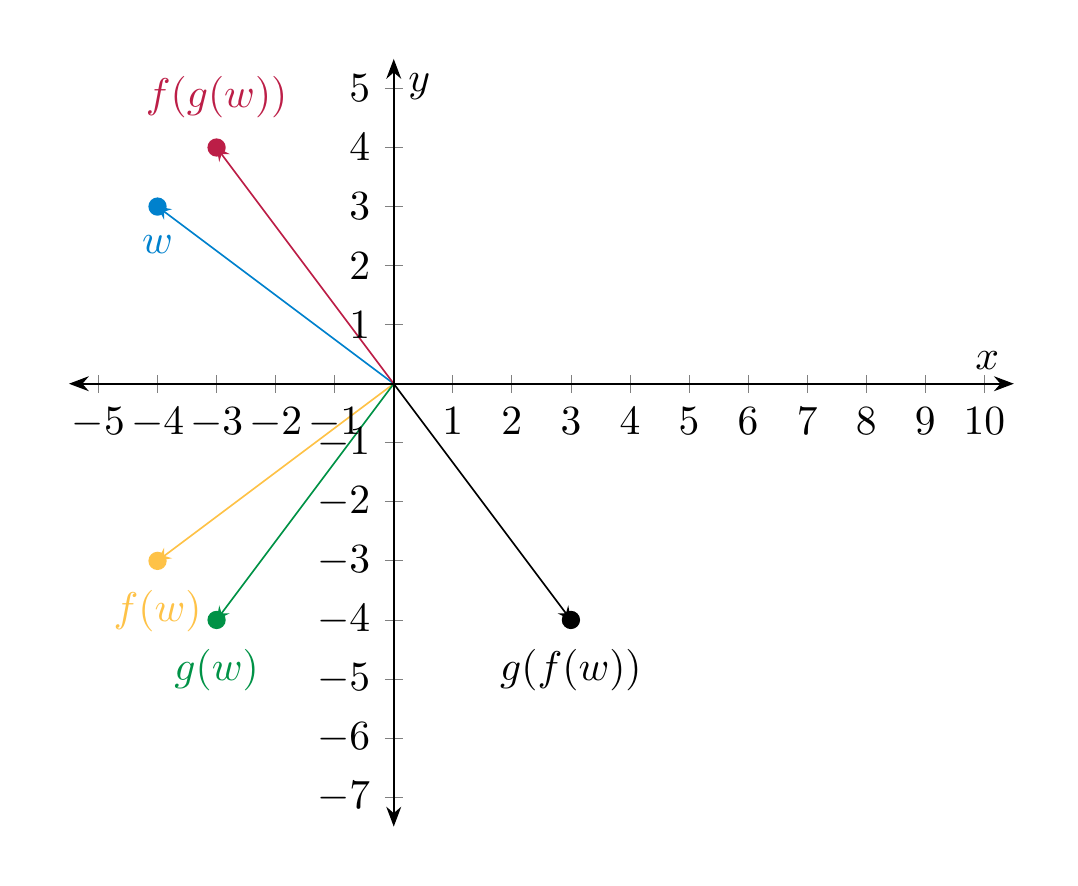
The phenomenon \(AB \ne BA\) may be best understood in the light of composition of (linear) maps: if \(f : {\bf R}^n \to {\bf R}^n\) and \(g : {\bf R}^n \to {\bf R}^n\) is another linear map, then in general we have

\[ g \circ f \ne f \circ g. \]

To take a concrete example, consider the linear map \(f : {\bf R}^2 \to {\bf R}^2\) given by reflecting along the \(x\)-axis, and \(g : {\bf R}^2 \to {\bf R}^2\) the linear map given by rotating counter-clockwise (around the origin) by \(90^\circ\).

Let us conclude this discussion by noting that this issue is not specific to linear algebra, but is a common phenomenon in daily life: there is (often) no reason to expect that doing (the same) two actions in different order give the same result:

• You first do sports, then take a shower.

• You first take a shower, then do sports.

In the first scenario you may feel refreshed, in the second one a little sweaty...

Further properties of matrix multiplication

Definition 4.58 (Related exercises: Exercise 4.25)

The identity matrix is the square matrix

\[ {\mathrm {id}} = \left ( \begin{array}{cccc} 1 & 0 & \dots & 0 \\ 0 & 1 & \dots & 0 \\ \vdots & & \ddots & \vdots \\ 0 & \dots & 0 & 1 \end{array} \right ). \]

I.e., it is a square matrix whose entries on the “north-west – south-east” diagonal (which is called the main diagonal) are all 1, and the remaining entries are zero. If it is important to specify the size, one also writes \({\mathrm {id}}_n\).

Example 4.59

If \(n=1\), then \({\mathrm {id}}_1\) is just the \(1 \times 1\)-matrix whose only entry is 1. \({\mathrm {id}}_2 = \left ( \begin{array}{cc} 1 & 0 \\ 0 & 1 \end{array} \right )\).

The first two identities in the next lemma assert that the identity matrix takes the role of the number 1 when it comes to multiplying matrices.

Lemma 4.60 (Related exercises: Exercise 6.10, Exercise 4.41, Exercise 4.25, Exercise 4.20)

Matrix multiplication satisfies the following identities, where \(A\), \(B\) and \(C\) are matrices (of a size such that the products and sums below are defined), and \(r \in {\bf R}\):

\[ \begin{align*} {\mathrm {id}} A & = A \\ A {\mathrm {id}} & = A \\ A (B+C) & = AB + AC & \text{(distributivity)} \\ (A+B) C &= AC + BC \\ (AB)C &= A(BC) & \text{(associativity)} \\ r(AB) &= (rA)B = A (rB) & \text{(matrix vs.~scalar multiplication)} \end{align*} \]

Proof. These identities follow from similar identities for the multiplication and addition of real numbers.

To illustrate the principle, we consider the first distributivity law above. Let \(A = (a_{ij})\) be an \(m \times n\)-matrix and \(B, C\) two \(n \times k\)-matrices, \(B = (b_{ij})\) and \(C = (c_{ij})\). Then \(B+C = (b_{ij}+c_{ij})\) so that

\[ \begin{align*} A(B+C) & = (\sum_{e = 1}^n a_{ie} (b_{ej} + c_{ej})) \\ & \stackrel ! = (\sum_{e = 1}^n a_{ie} b_{ej} + a_{ie} c_{ej}) \\ & = (\sum_{e = 1}^n a_{ie} b_{ej}) + (\sum_{e=1}^n a_{ie} c_{ej}) \\ & = AB + AC. \end{align*} \]

At the equality marked ! we have used the distributivity law for real numbers, i.e., the identity \(e(f+g) = ef+eg\) for any \(e, f, g \in {\bf R}\). ◻

Multiplication with elementary matrices

We recast the elementary row operations of matrices (Definition 2.28) in terms of multiplication with appropriate matrices. Below, we use the (standard) convention that an “invisible” entry in a matrix is zero, e.g. \({\mathrm {id}}_2 = \left ( \begin{array}{cc} 1 & 0 \\ 0 & 1 \end{array} \right )\) will be written as \(\left ( \begin{array}{cc} 1 & {} \\ {} & 1 \end{array} \right )\) etc.

Proposition 4.61

Let \(A\) be an \(m \times n\)-matrix.

1. Let \(A'\) be the matrix obtained by interchanging the \(i\)-th and the \(j\)-th row. Then

\[ A' = \underbrace{\left ( \begin{array}{ccccccc} 1 & & & & & & \\ & \ddots & & & & & \\ & & 0 & & 1 & & \\ & & & \ddots & & & \\ & & 1 & & 0 & & \\ & & & & & \ddots & \\ & & & & & & 1 \end{array} \right )}_{E^{(1)}_{i,j}} A. \]

(The first matrix is the \(m \times m\)-matrix obtained from \({\mathrm {id}}_m\) by exchanging the \(i\)-th and the \(j\)-th row.)

1. Let \(A'\) be the matrix obtained by multiplying the \(i\)-th row with a real number \(r\). Then

\[ A' = \underbrace{\left ( \begin{array}{ccccccc} 1 & & & & & & \\ & \ddots & & & & & \\ & & 1 & & & & \\ & & & r & & & \\ & & & & 1 & & \\ & & & & & \ddots & \\ & & & & & & 1 \end{array} \right )}_{E^{(2)}_{i,r}} A . \]

(The first matrix is the \(m \times m\)-matrix obtained from \({\mathrm {id}}_m\) by replacing the \((i,i)\)-entry by \(r\).)

1. Let \(A'\) be the matrix obtained by adding the \(r\)-th multiple of the \(j\)-th row to the \(i\)-th row. Then

\[ A' = \underbrace{\left ( \begin{array}{ccccccc} 1 & & & & & & \\ & \ddots & & & & & \\ & & 1 & & & & \\ & & & \ddots & & & \\ & & r & & 1 & & \\ & & & & & \ddots & \\ & & & & & & 1 \end{array} \right )}_{E^{(3)}_{i,j,r}} A. \]

(The first matrix is the \(m \times m\)-matrix obtained from \({\mathrm {id}}_m\) by replacing the \((i,j)\)-entry by \(r\).)

Definition 4.62 (Related exercises: Exercise 4.20)

The matrices \(E^{(1)}_{i,j}\), \(E^{(2)}_{i,r}\) and \(E^{(3)}_{i,j,r}\) (for any appropriate \(i\), \(j\) and any \(r \in {\bf R}\), where \(r \ne 0\) in \(E^{(2)}_{i,r}\)) appearing in the statement above are called elementary matrices.

Proof. This is a more cumbersome to write down precisely than to convince oneself by unwinding the definition. We check the third statement. If \(B=(b_{ij})\) is the above matrix as stated, we have that \(b_{ii} = 1\) and \(b_{ij} = r\) and all other entries are zero. Let us write \(C = BA\), \(C = (c_{ij})\). Then, by definition,

\[ c_{st} = \sum_{e=1}^m b_{se} a_{et}. \]

We compute this sum:

• if \(s \ne i\), then the only \(b_{se}\) that is non-zero is \(b_{ss} = 1\), so that

\[ c_{st} = b_{ss} a_{st} = a_{st}. \]

• For \(s = i\), the only coefficients \(b_{se}\) that are non-zero are \(b_{ss} = 1\) and \(b_{sj} = r\). Thus, the sum above consists of two terms, and therefore

\[ c_{st} = b_{ss} a_{st} + b_{sj} a_{jt} = a_{st} + r a_{jt}. \]

Thus the \(i\)-th row of \(C\) equals the matrix \(A'\) as in the statement above. ◻