Revisiting linear systems

In this section, we apply our findings from above to the problem of solving a linear system

\[ \begin{align*} a_{11} x_1 + \dots + a_{1n} x_n & = b_1\\ \vdots \\ a_{m1} x_1 + \dots + a_{mn} x_n & = b_m \end{align*} \]

Throughout, let \(A = (a_{ij})\) be the \(m \times n\)-matrix formed by the coefficients of that linear system. Recall that the vector

\[ b := \left ( \begin{array}{c} b_1 \\ \vdots \\ b_m \end{array} \right ) \]

is called the vector of constants. We will also consider the linear map (Proposition 4.19)

\[ f : {\bf R}^n \to {\bf R}^m, v \mapsto Av. \]

Theorem 4.37 (Related exercises: Exercise 4.9, Exercise 4.14)

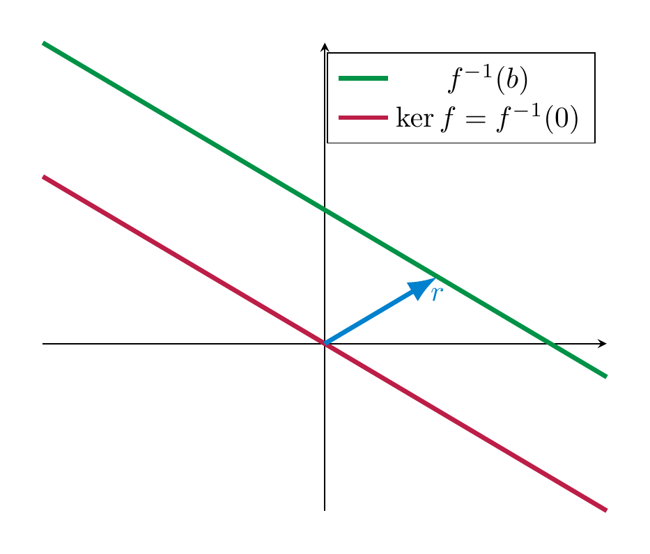
1. Suppose momentarily that \(b_1 = \dots = b_m = 0\), so the above system is homogeneous. In this case the solution set equals \(\ker f\), which in particular is a subspace of \({\bf R}^n\).

2. For arbitrary \(b\), the system above has (at least) one solution if the vector \(b\) lies in the image of \(f\). (Note that the vector is \({\bf R}^m\), and \({\operatorname{im}\ } f \subset {\bf R}^m\).) If \(r = (r_1, \dots, r_n)\) is any such solution, then the solution set consists precisely of the vectors of the form

\[ r + \ker f := \{r + v, \text{ where } v \in \ker f\}. \]

Proof. Recall from Observation 4.11 that

\[ f^{-1}(b) = \{ r \in {\bf R}^n \ | \ A r = b \} \]

consists precisely of the solutions of the system above.

Therefore, the first statement is clear: \(\ker f = f^{-1}(0)\) are the solutions of the homogeneous system. Also, the (non-homogeneous) system has a solution precisely if \(f^{-1}(b)\) is non-empty, i.e., if \(b \in {\operatorname{im}\ } f\). For the last statement: we show both implications:

• if \(s = (s_1, \dots, s_n)\) is a solution, then we get

\[ f(s-r) = f(s) - f(r) \]

since \(f\) is linear. Since \(r\) is some solution of the system, we have \(f(r) = b\), and also \(f(s) = b\). This implies \(v := s-r \in \ker f\), i.e., \(s = r + v\).

• Conversely, consider a vector of the form \(r + v\), with \(v \in \ker f\). Then

\[ f(r+v) = f(r) + f(v) = b + 0 = b. \]

Thus \(r+v\) is also a solution of the system.

◻

Remark 4.38 (Related exercises: Exercise 4.9, Exercise 4.14)

The solution set \(r + \ker f\) of a non-homogeneous system is never a subspace: indeed any subspace contains the zero vector, but if that is a solution we get

\[ b = A 0 = 0. \]

Instead, the solution set of the system with a non-zero vector \(b\), i.e., \(f^{-1}(b)\) is a translation of \(\ker f\), as is

Example 4.39

Consider the linear system (in the unknowns \(x, y, z\))

\[ \begin{align*} x + 3y+5z & = 7 \\ 3x+9y+10z & = 11 \\ 2x+ 9y+12 z & = 10. \end{align*} \]

The pertinent \(3 \times 3\)-matrix built out of the coefficients is

\[ A = \left ( \begin{array}{ccc} 1 & 3 & 5 \\ 3 & 9 & 10 \\ 2 & 9 & 12 \end{array} \right ). \]

As above, we write \(f : {\bf R}^3 \to {\bf R}^3, v = \left ( \begin{array}{c} x \\ y \\ z \end{array} \right ) \mapsto A v\) for the associated linear map.

We compute its rank by bringing it into row-echelon form:

\[ A \leadsto \left ( \begin{array}{ccc} 1 & 3 & 5 \\ 0 & 0 & -5 \\ 0 & 3 & 2 \end{array} \right ) \leadsto \left ( \begin{array}{ccc} 1 & 3 & 5 \\ 0 & 0 & 1 \\ 0 & 3 & 2 \end{array} \right ) \leadsto \left ( \begin{array}{ccc} 1 & 3 & 5 \\ 0 & 0 & 1 \\ 0 & 1 & 0 \end{array} \right ) \stackrel{\text{swap}} \leadsto \left ( \begin{array}{ccc} 1 & 3 & 5 \\ 0 & 1 & 0 \\ 0 & 0 & 1 \end{array} \right ) . \]

This matrix has 3 leading ones, hence its rank is 3. Thus, \(f\) is surjective. By the rank-nullity theorem we have

\[ \dim \ker f = \dim {\bf R}^3 - \dim {\operatorname{im}\ } f = 3 - 3 = 0. \]

Therefore, \(f\) is injective (Lemma 4.25). (Alternatively, we may use Corollary 4.285. directly to see \(f\) is injective.) Thus, \(f\) is bijective. This means that for any vector of constants, such as the above \(\left ( \begin{array}{c} 7 \\ 11 \\ 10 \end{array} \right )\), there is precisely one solution of the linear system. This solution can be determined via Method 2.31, but we will omit this computation here because we will later develop a more comprehensive method, namely by using the inverse \(A^{-1}\), to obtain these solutions.