Eigenspaces

In the above examples, the set of all eigenvectors for a given eigenvalue has a particularly nice shape. This is a general phenomenon:

Definition and Lemma 6.11

Let \(A \in {\mathrm {Mat}}_{n \times n}\) be a square matrix and \(\lambda \in {\bf R}\) a fixed real number. The set

\[ E_\lambda := \{ v \in {\bf R}^n \ | \ A v = \lambda v \} \]

is a subspace of \({\bf R}^n\). It is called the eigenspace of \(A\) with respect to \(\lambda\).

Proof. The equation \(Av = \lambda v\) is equivalent to \((A - \lambda {\mathrm {id}})v = 0\), i.e., we have \(E_\lambda = \ker (A - \lambda {\mathrm {id}})\). This is a subspace of \({\bf R}^n\) by Proposition 4.23. ◻

Remark 6.12

If \(\lambda\) above is not an eigenvalue, then \(E_\lambda = \{ 0 \}\), i.e., the zero vector is the only one satisfying \(Av = \lambda v\).

If \(\lambda\) is an eigenvalue, then \(E_\lambda\) consists of all the eigenvectors for the eigenvalue \(\lambda\), together with the zero vector (which by definition is not an eigenvector).

Example 6.13

We compute the eigenspaces of the matrix \(A = \left ( \begin{array}{cc} 0 & -1 \\ -2 & 0 \end{array} \right )\). Its characteristic polynomial is

\[ \chi_A(t)=\det \left ( \begin{array}{cc} -\lambda & -1 \\ -2 & -\lambda \end{array} \right ) = \lambda^2 - 2. \]

Its zeros, i.e., the eigenvalues of \(A\) are \(\lambda_{1/2} = \pm \sqrt 2\). The eigenspace for \(\sqrt 2\) is the solution space of the homogeneous system

\[ \underbrace{\left ( \begin{array}{cc} -\sqrt 2 & -1 \\ -2 & -\sqrt 2 \end{array} \right )}_{= A - \sqrt 2 \cdot {\mathrm {id}} =: B} \left ( \begin{array}{c} x \\ y \end{array} \right ) = 0. \]

We solve this by reducing the matrix \(B\) to row-echelon form

\[ \left ( \begin{array}{cc} -\sqrt 2 & -1 \\ -2 & -\sqrt 2 \end{array} \right ) \leadsto \left ( \begin{array}{cc} 1 & \frac 1{\sqrt 2} \\ -2 & -\sqrt 2 \end{array} \right ) \leadsto \left ( \begin{array}{cc} 1 & \frac {\sqrt 2}2 \\ 0 & 0 \end{array} \right ). \]

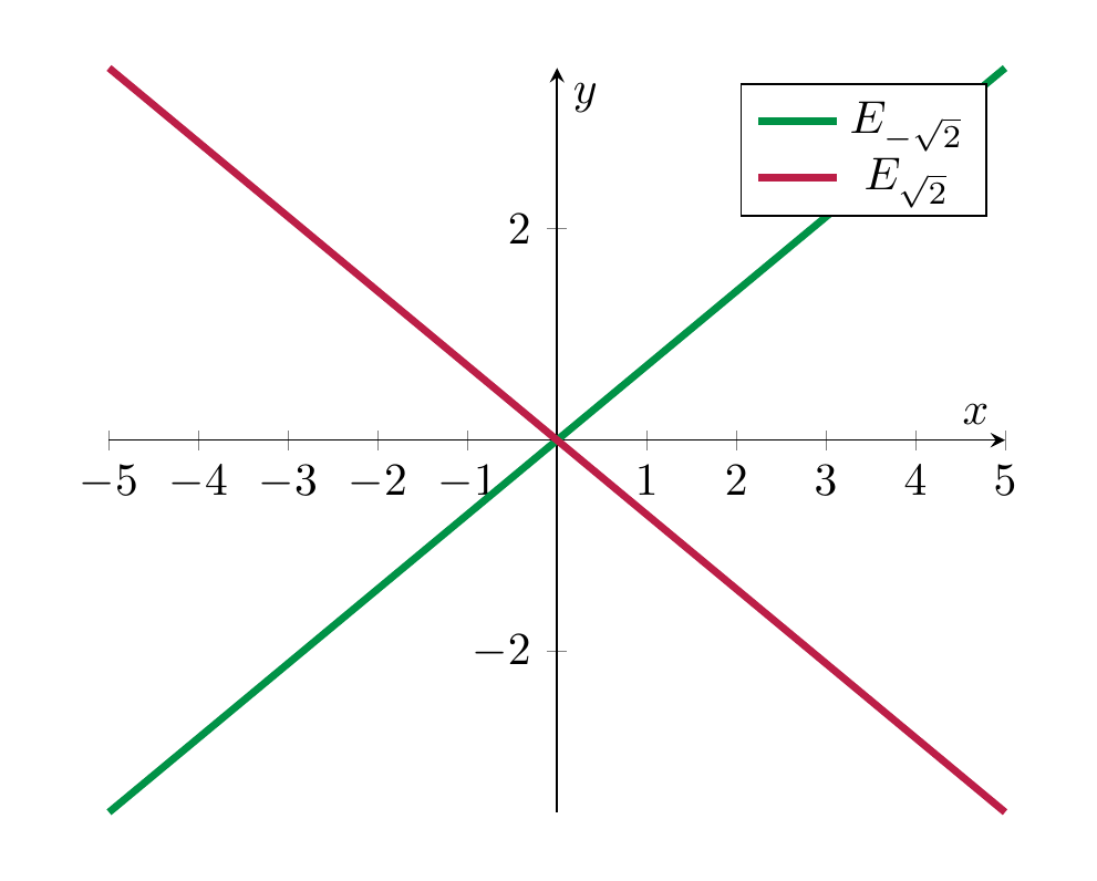
Thus, \(y\) is a free variable and \(x = - \frac{\sqrt 2}2 y\). Thus \(E_{\sqrt 2}\) has dimension 1, a basis vector is \((-\frac{\sqrt 2}2, 1)\). Similarly, one computes the eigenspace for \(\lambda = -\sqrt 2\):

\[ B = A + \sqrt 2 \cdot {\mathrm {id}} = \left ( \begin{array}{cc} \sqrt 2 & -1 \\ -2 & \sqrt 2 \end{array} \right ) \leadsto \left ( \begin{array}{cc} 1 & -\frac{1}{\sqrt 2} \\ -2 & \sqrt 2 \end{array} \right ) \leadsto \left ( \begin{array}{cc} 1 & -\frac{\sqrt 2}{2} \\ 0 & 0 \end{array} \right ), \]

so the eigenspace \(E_{-\sqrt 2}\) is again one-dimensional, and a basis vector is \((\frac{\sqrt 2}2, 1)\). Here is a plot showing the two eigenspaces: the map \(v \mapsto Av\) will stretch the vectors in \(E_{\sqrt 2}\) by a factor of \(\sqrt 2\), while those on the eigenspace \(E_{-\sqrt 2}\) will be flipped and stretched by a factor of \(\sqrt 2\):