Euclidean spaces

The definition of a (real) vector space encodes the existence (and good properties) of the addition of vectors and the scalar multiplication of vectors. The vector space \({\bf R}^n\) has, however, another important piece of structure, namely the distance between two points, and the property of vectors being orthogonal to each other.

The scalar product on \({\bf R}^n\)

Definition 7.1

The scalar product of \(v, w \in {\bf R}^n\) is defined as

\[ {\left \langle v, w \right \rangle} := v^T {\mathrm {id}} w = v^T w = v_1 w_1 + \dots + v_n w_n. \]

(This is not to be confused with the scalar multiple of a vector, which is again a vector!)

Example 7.2

The scalar product can be positive, zero, or negative:

• \({\left \langle \left ( \begin{array}{c} 1 \\ 2 \end{array} \right ), \left ( \begin{array}{c} -2 \\ 2 \end{array} \right ) \right \rangle} = 1 \cdot (-2) + 2 \cdot 2 = 2\)

• \({\left \langle \left ( \begin{array}{c} 1 \\ 2 \end{array} \right ), \left ( \begin{array}{c} -2 \\ 1 \end{array} \right ) \right \rangle} = 1 \cdot (-2) + 2 \cdot 1 = 0\)

• \({\left \langle \left ( \begin{array}{c} 1 \\ 2 \end{array} \right ), \left ( \begin{array}{c} -2 \\ 0 \end{array} \right ) \right \rangle} = 1 \cdot (-2) + 2 \cdot 0 = -2\)

However, for any \(v \in {\bf R}^n\), we have

\[ {\left \langle v, v \right \rangle} = \sum_{i=1}^n v_i^2 \ge 0 \]

(7.3)

i.e., a scalar product of a vector with itself is always non-negative. This implies that

\[ |\hspace{-0.5mm}| {v} |\hspace{-0.5mm}| := \sqrt{\left \langle v, v \right \rangle} = \sqrt{v_1^2 + \dots + v_n^2} \]

is a well-defined (real) number. It is called the norm of the vector \(v\).

Lemma 7.4

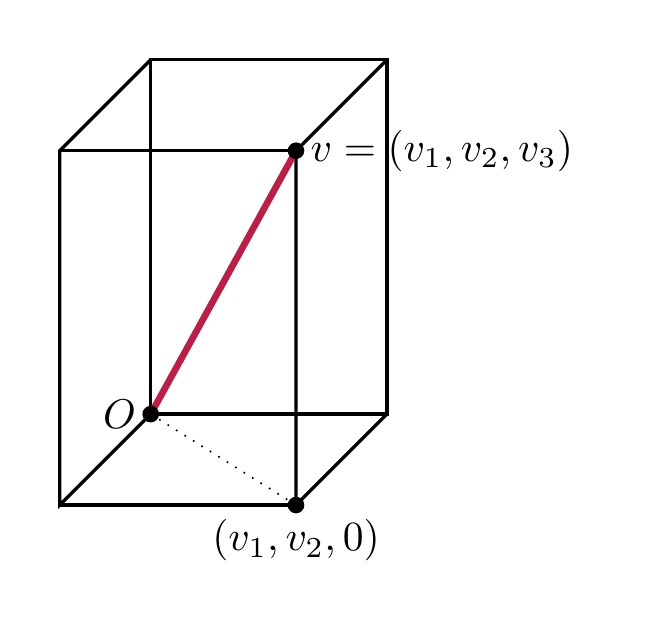
The norm \(|\hspace{-0.5mm}| {v} |\hspace{-0.5mm}|\) is the length of the line segment from the origin to \(v\).

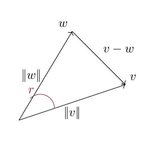
For \(v, w \in {\bf R}^2\), there holds

\[ {|\hspace{-0.5mm}| {v-w} |\hspace{-0.5mm}|}^2 = |\hspace{-0.5mm}| {v} |\hspace{-0.5mm}|^2 + |\hspace{-0.5mm}| {w} |\hspace{-0.5mm}|^2 - 2 |\hspace{-0.5mm}| {v} |\hspace{-0.5mm}| |\hspace{-0.5mm}| {w} |\hspace{-0.5mm}| \cos r, \]

where \(r\) is the angle between the vector \(v\) and \(w\).

Proof. The formula for the norm follows from repeatedly applying the Pythagorean theorem. Illustrating this for \(n = 3\), we see that the line segment (shown dotted below) from the origin \(O = (0,0,0)\) to the point \((v_1, v_2, 0)\) has length \(\sqrt{v_1^2 + v_2^2}\). Therefore the length of the segment from \(O\) to \(v\) is

\[ \sqrt{\left (\sqrt{v_1^2 + v_2^2} \right)^2 + v_3^2} = \sqrt{v_1^2 + v_2^2 + v_3^2}. \]

The formula for the norm of \(v-w\) follows is a reformulation of the law of cosines.

◻

Given a square matrix \(A \in {\mathrm {Mat}}_{n \times n}\), we have considered so far the linear map

\[ {\bf R}^n \to {\bf R}^n, v\mapsto A \cdot v. \]

In addition to that, there is another fundamental map that one can associate to a matrix:

\[ {\left \langle -, - \right \rangle_{A}} : {\bf R}^n \times {\bf R}^n \to {\bf R}, (v, w) \mapsto {\left \langle v, w \right \rangle_{A}} := v^T \cdot A \cdot w. \]

Here we regard \(v\) and \(w\) as column vectors, i.e., as \(n \times 1\)-matrices. Therefore, for \(v = \left ( \begin{array}{c} v_1 \\ \vdots \\ v_n \end{array} \right )\), \(v^T = \left ( \begin{array}{ccc} v_1 & \dots & v_n \end{array} \right )\) is a row vector (with \(n\) entries). Therefore \(v^T A\) is an \(1 \times n\)-matrix, so that \(v^T A w\) is an \(1 \times 1\)-matrix, i.e., just a real number. We call this number the scalar product of \(v\) and \(w\) with respect to the given matrix \(A\).

Lemma 7.5 (Related exercises: Exercise 7.1)

The scalar product has the following fundamental properties:

• If we fix \(w \in {\bf R}^n\), then the maps

\[ \begin{align*} {\left \langle ?, w \right \rangle} : & {\bf R}^n \to {\bf R}, v \mapsto {\left \langle v, w \right \rangle}\\ {\left \langle w, ? \right \rangle} : & {\bf R}^n \to {\bf R}, v \mapsto {\left \langle w, v \right \rangle} \end{align*} \]

are linear (cf. Definition 4.1; e.g., for the first this means concretely that

\[ {\left \langle rv+r'v', w \right \rangle} = r{\left \langle v, w \right \rangle} + r'{\left \langle v', w \right \rangle}, \]

for \(r, r' \in {\bf R}\), \(v, v' \in {\bf R}^n\). We refer to this by saying that \({\left \langle -, - \right \rangle} : {\bf R}^n \times {\bf R}^n \to {\bf R}\) is a bilinear form (or as the bilinearity of the scalar product).

• We have

\[ {\left \langle v, w \right \rangle} = {\left \langle w, v \right \rangle}. \]

This property is called symmetry.

Proof. By Proposition 4.19, the map \(w \mapsto v^T w = {\left \langle v, w \right \rangle}\) is linear. The proof of the linearity in the first argument is similar, or it follows from symmetry.

The identity \({\left \langle v, w \right \rangle} = {\left \langle w, v \right \rangle}\) is directly clear from the definition. One may also prove it using :

\[ (v^T w)^T = w^T (v^T)^T = w^T v. \]

Noting that any \(1 \times 1\)-matrix (such as \(v^T w\)) is equal to its transpose, the left hand side equals \({\left \langle v, w \right \rangle}\), while the right equals \({\left \langle w, v \right \rangle}\). ◻

Using the bilinearity of \({\left \langle -, - \right \rangle}\), we can compute the following expression

\[ \begin{align*} {|\hspace{-0.5mm}| {v-w} |\hspace{-0.5mm}|}^2 & = {\left \langle v-w, v-w \right \rangle} \\ & = {\left \langle v, v-w \right \rangle} - {\left \langle w, v-w \right \rangle} \\ & = {\left \langle v, v \right \rangle} - {\left \langle v, w \right \rangle} - {\left \langle w, v \right \rangle} + {\left \langle w, w \right \rangle} \\ & = {|\hspace{-0.5mm}| {v} |\hspace{-0.5mm}|}^2 + {|\hspace{-0.5mm}| {w} |\hspace{-0.5mm}|}^2 - 2 {\left \langle v, w \right \rangle}. \end{align*} \]

Comparing this with the cosine law above we see

\[ {\left \langle v, w \right \rangle} = |\hspace{-0.5mm}| {v} |\hspace{-0.5mm}| |\hspace{-0.5mm}| {w} |\hspace{-0.5mm}| \cos r. \]

The factor \(\cos r\) is equal to 0 precisely if \(r = -\frac \pi 2, \frac \pi 2\) (i.e., \(90^\circ\) or \(-90^\circ\)). In other words,

\[ {\left \langle v, w \right \rangle} = 0 \]

if the angle between the vectors \(v\) and \(w\) is \(\pm 90^\circ\). This motivates the following definition.

Definition 7.6

Two vectors \(v, w \in {\bf R}^n\) are said to be orthogonal if

\[ {\left \langle v, w \right \rangle} = \sum_{i=1}^n v_i w_i = 0. \]

Positive definite matrices

Definition and Lemma 7.7

If \(A\) is a symmetric \(n \times n\)-matrix (i.e., \(A = A^T\)), then the map

\[ {\left \langle -, - \right \rangle_{A}} : {\bf R}^n \times {\bf R}^n \to {\bf R}, {\left \langle v, w \right \rangle_{A}} := v^T A w \]

is bilinear and symmetric, i.e., Lemma 7.5 holds verbatim for \({\left \langle -, - \right \rangle_{A}}\) instead of the standard scalar product (which corresponds to the case \(A = {\mathrm {id}}_n\)).

Example 7.8

Suppose \(A = \left ( \begin{array}{cccc} 1 & 0 & 0 & 0 \\ 0 & 1 & 0 & 0 \\ 0 & 0 & 1 & 0 \\ 0 & 0 & 0 & -1 \end{array} \right )\). Then \(A w = \left ( \begin{array}{c} w_1 \\ w_2 \\ w_3 \\ -w_4 \end{array} \right )\), so that

\[ \begin{align*} {\left \langle v, w \right \rangle_{A}} & = v^T A w = \left ( \begin{array}{cccc} v_1 & v_2 & v_3 & v_4 \end{array} \right ) \cdot \left ( \begin{array}{c} w_1 \\ w_2 \\ w_3 \\ -w_4 \end{array} \right ) \\ & = v_1 w_1 + v_2 w_2 +v_3w_3 - v_4 w_4. \end{align*} \]

This example is not an anomaly, but the basis of so-called Minkowski space which is fundamental in special relativity, which is \({\bf R}^{3+1}\) with 3 space coordinates and 1 time coordinate.

The standard basis vectors \(e_1 = \left ( \begin{array}{c} 1 \\ 0 \\ 0 \\ 0 \end{array} \right ), \dots, e_4 = \left ( \begin{array}{c} 0 \\ 0 \\ 0 \\ 1 \end{array} \right )\) are orthogonal to each other, but

\[ {\left \langle e_4, e_4 \right \rangle_{A}} = -1 \]

where as \({\left \langle e_k, e_k \right \rangle_{A}} = +1\) for the other three basis vectors. In that sense, the scalar product (with respect to \(A\)) is able to distinguish between the last and the other three directions.

Definition 7.9

A symmetric matrix \(A\) is called positive definite if

\[ {\left \langle v, v \right \rangle_{A}} > 0 \]

for all \(v \in {\bf R}^n\), \(v \ne 0\). In this case we can define the norm (of \(v\) with respect to the matrix \(A\)) as

\[ {|\hspace{-0.5mm}| {v} |\hspace{-0.5mm}|}_{A} := \sqrt {\left \langle v, v \right \rangle_{A}}. \]

It is negative definite if instead \({\left \langle v, v \right \rangle_{A}} < 0\) for all \(v \ne 0\). The matrix \(A\) is called indefinite if there exist \(v, w \in {\bf R}^n\) with \({\left \langle v, v \right \rangle_{A}} > 0\) and \({\left \langle w, w \right \rangle_{A}} < 0\).

Example 7.10

As we have seen in , \({\mathrm {id}}_n\) is positive definite. The matrix in Example 7.8 is indefinite.

It is suggestive to blame the \(-1\) in the last entry for the indefiniteness of the matrix in Example 7.8. The following result gives a way to ensure positive definiteness for general matrices. To state it, we introduce a bit of terminology:

Definition 7.11

For a square matrix \(A\), the principal submatrix (of size \(r\)) is the matrix

\[ A^{(r)} = (a_{ij})_{1 \le i, j \le r}. \]

I.e., it is the matrix consisting of the first \(r\) rows and columns of \(A\).

Proposition 7.12

Let \(A \in {\mathrm {Mat}}_{n \times n}\) be a symmetric square matrix. The following are equivalent:

1. the bilinear form \({\left \langle -, - \right \rangle_{A}}\) is positive definite, i.e., \({\left \langle v, v \right \rangle_{A}} \ge 0\) for all \(v \in {\bf R}^n\),

2. \(A\) is positive definite,

3. For all \(1 \le r \le n\), \(\det (A^{(r)}) > 0\).

In particular, any positive definite matrix \(A\) has \(\det A > 0\). Therefore such a matrix is invertible (Theorem 5.15).

A proof of this criterion requires methods from §Section 7.3.

Example 7.13

Consider the matrix \(A = \left ( \begin{array}{ccc} 1 & 2 & t \\ 2 & 5 & 8 \\ t & 7 & 14 \end{array} \right )\), where \(t \in {\bf R}\) is some parameter. We inspect its positive definiteness: since \(A^{(1)} = 1\) is positive, \(\det A^{(2)} = \det \left ( \begin{array}{cc} 1 & 2 \\ 2 & 5 \end{array} \right ) = 1 > 0\) and \(\det A = \det A^{(3)} = -5t^2 + 32t -50\). For \(t = 3\), this equals \(+1\), so the matrix \(A\) is positive definite in this case. For \(t=4\), this equals \(-2\), so the matrix \(A\) is indefinite in this case.

Example 7.14

The defininiteness of matrices has applications in analysis: for a (twice differentiable) function \(f : {\bf R}^2 \to {\bf R}\), such as

\[ f(x,y)= x^2 + y^2, \]

one considers the so-called Hesse matrix, which is given by

\[ \left ( \begin{array}{cc} \frac{\partial^2 f}{\partial x \partial x} & \frac{\partial^2 f}{\partial x \partial y} \\ \frac{\partial^2 f}{\partial y \partial x} & \frac{\partial^2 f}{\partial y \partial xy} \end{array} \right ). \]

For the above function it is

\[ \left ( \begin{array}{cc} 2 & 0 \\ 0 & 2 \end{array} \right ), \]

which is positive definite. By contrast, for \(g(x, y)=x^2 - y^2\), it is \(\left ( \begin{array}{cc} 2 & 0 \\ 0 & -2 \end{array} \right )\), which is indefinite. One proves in analysis that the positive defininetess of the Hesse matrix implies that there is a local minimum at a given point \((x,y)\), provided that \(\frac{\partial f}{\partial x} = \frac{\partial f}{\partial y} = 0\) at this point. Thus, \(f\) has a local minimum at the point \((0,0)\), but \(g\) does not.

The function g(x, y) = x² − y² has a saddle point at (0, 0); informally this means that there are directions in which g increases (here the x-direction, shown blue), and directions in which g decreases (the y-direction, red parabola).

The function f(x, y) = x² + y² has a local minimum at (0, 0). Informally this means that moving in any direction from the point (0, 0), the value of f(x, y) increases.